The Rasch model
What this is for
Sum scores treat every item as interchangeable: a correct answer is worth one point no matter which item it came from. Yet items differ, and the chance of getting any one of them right does not rise in a straight line with the sum score (Where CTT breaks). What is the simplest model that takes items seriously? The Rasch model (Rasch, 1960), with one parameter per person and one per item, on the same scale. That parsimony buys some unusual properties, chief among them that the sum score is all the model needs to know about a person, and it makes demands of the data. This lesson is about both.
Goals
By the end of this lesson you should be able to:
- write down the Rasch model and say what \(\theta\) and \(b\) mean;
- read an item characteristic curve and a Wright map;
- explain why the scale has no natural origin (and what software does about it);
- explain why the sum score is all the Rasch model needs to know about a person, and what “specific objectivity” asks of the data;
- fit the model to real item response data with
mirt, and read item fit statistics and plots to judge where it fits and where it doesn’t.
Core ideas
From logistic regression to the Rasch model
The Rasch model answers it, and takes the step Where CTT breaks pointed to. It keeps the shape of the logistic regression, but everything on the right-hand side is unknown. For person \(j\) and item \(i\), \[\Pr(x_{ij} = 1) = \frac{\exp(\theta_j - b_i)}{1 + \exp(\theta_j - b_i)}.\]
- \(\theta_j\) is the person’s ability, an idealized version of the sum score. It, and it alone, determines how a person performs on the items. It takes the place of \(\beta_1 \times \text{Elo}\), or of the sum score in the item curves.
- \(b_i\) is the item’s difficulty, the item intercept with its sign flipped. When \(\theta = b\), the odds of a correct response are even.
Plotting the probability of a correct response against \(\theta\) for a single item gives the item characteristic curve (ICC): the item curve of Where CTT breaks, with \(\theta\) where the sum score was. Move the difficulty around and watch what happens.
Try it: an item characteristic curve
Changing \(b\) slides the curve left and right without changing its shape: a harder item needs more ability for the same chance of success. The curve never reaches 0 or 1, so nobody is certain to get any item right or wrong. The Rasch model fixes the slope at 1 for every item; letting it vary gives the 2PL of From the 1PL to the 4PL.
The scale has no origin
Where is zero on this scale? Nowhere in particular. Add the same constant \(C\) to every ability and every difficulty: the model only ever sees \(\theta - b\), so no predicted response changes.
Try it: shift everything
The probabilities in the last column do not move. The data say how far apart people and items are, but not where zero is: without an extra constraint the model is not identified. Software picks one for you. mirt (Chalmers, 2012) fixes the mean of the ability distribution at 0, as the chess fit below shows. Programs that use conditional maximum likelihood (see the Go deeper callout below) instead fix one item’s difficulty at 0 or make the difficulties sum to 0 (Mair & Hatzinger, 2007). The choice is arbitrary, so two programs’ results can differ by exactly such a shift.
People and items on one scale: the Wright map
In the Rasch model a person’s location is \(\theta\), not a count of items, and \(\theta\) and \(b\) live on the same scale, so we can plot them together. A Wright map puts the distribution of people on one side and the item difficulties on the other, and shows at a glance whether a test is well matched to the people who took it.
Try it: build a Wright map
Where people and items overlap, the test can tell people apart; where people sit beyond every item, it cannot. That precision depends on where you are on the scale is the subject of Information, precision, and short forms.
What the model assumes
Two assumptions merit emphasis (Lord, 1980). First, the formula is right: in particular, a single \(\theta\) drives every response (the model is unidimensional). Second, responses are locally independent: once we know \(\theta\), knowing how someone answered item 3 tells us nothing more about item 4. Both can fail: think of two items that share a reading passage, or a test whose last ten items measure something else. IRW vignettes look at how often each assumption holds across many IRW datasets: dimensionality and local dependence.
The sum score is sufficient
The Rasch model has a property that sets it apart from nearly every other item response model: the sum score \(r\) is a sufficient statistic for \(\theta\) (Fisher, 1922). Once you know how many items someone got right, nothing else in their responses, not even which items, changes what we can learn about their ability.
For one respondent, \(\theta\) plays the part of that intercept. So the maximum-likelihood estimate of \(\theta\) is the value at which the expected number correct, \(\sum_i \Pr(x_i = 1 \mid \theta)\), equals the observed number correct, \(r\). Which items make up \(r\) never enters the equation.
Below are five items of increasing difficulty. Pick a response pattern and look at the likelihood for \(\theta\); then look at every other pattern with the same sum score.
Try it: sufficiency
Under the Rasch model the column is constant. Switch to the 2PL and it no longer is: getting a highly discriminating item right now counts for more. The relationship between sum scores and Rasch abilities is one-to-one but not linear. On these five items the step from 3 to 4 correct moves the estimate from 0.50 to 1.67, and 5 of 5 has no finite estimate at all.
So which to report, the sum score or \(\hat\theta\)? It rests on two assumptions. In the case that the Rasch model fits and everyone took the same items, the sum score carries everything the model knows about the respondent, it orders people exactly as \(\hat\theta\) does, and nobody needs it explained, so it may be sufficient for many purposes. When respondents take different items, as in Linking and equating, the sum scores are no longer comparable and \(\theta\) is. Whether the Rasch model fits well enough is itself something the data can answer, by setting it against its rivals on held-out responses (Model fit and out-of-sample prediction).
Specific objectivity
The Rasch tradition has a name for the property it prizes: specific objectivity (Rasch, 1977). Comparisons between people should not depend on which items we happened to use, and comparisons between items should not depend on which people happened to take them. It is a demand we place on the data, not something the data grants us for free.
If two items’ curves never cross, then everyone finds item A easier than item B, whatever their ability. If they cross, the ordering of the items depends on who you ask—and the statement “item A is easier than item B” stops meaning anything on its own.
Try it: do the curves cross?
This is why advocates of the Rasch model hold to it so firmly: specific objectivity and sufficiency are what classical measurement in the physical sciences looks like (Wright, 1997). The catch is that the model has to fit. In that tradition, consistency with the Rasch model comes from hard work—iterative item development and pruning of items that don’t behave—not from applying it to whatever data you have. Whether equal slopes are plausible for typical test data is an empirical question, and the 2PL discrimination vignette looks at it across many IRW datasets.
A note on estimation
Nothing on the right-hand side is known, so fitting takes two steps. mirt estimates the item parameters first, integrating over the distribution of abilities with the EM algorithm (Bock & Aitkin, 1981), then estimates abilities with those item parameters treated as known. Conditional maximum likelihood (Go deeper, above) is the Rasch model’s own alternative. Estimating abilities and Estimating item parameters take these in turn.
Simulate
The code below simulates responses from the Rasch model, fits the model with mirt, and compares the estimated difficulties to the truth. It runs here in your browser; the first run takes about 20 seconds while R and mirt load.
Try changing np to 50, then to 2000, and watch the scatter around the line. With the seed as written, the root mean squared error of the estimated difficulties is 0.34 with 50 people, 0.13 with 500 and 0.04 with 2,000. Now change ni to 40: with 500 people the error barely moves (0.13), because each difficulty rests on the people who answered that item. More items sharpen the abilities instead, which is where Information, precision, and short forms picks up.
mirt writes the Rasch model as \(\Pr(x = 1) = 1/(1 + \exp(-(\theta + d)))\), so its parameter d is an easiness. Our difficulty is \(b = -d\), which is why the code negates it.
Download this code to run it as large as you like in your own R session.
With real data
Our main example is chess_lnirt, the 40 problems of the Amsterdam Chess Test (van der Maas & Wagenmakers, 2005), which we met in The likelihood and logistic regression; its job here is to show what the Rasch model says about a test built for a wide range of skill. A response is 1 if the player solved the problem; download the code behind every number below.
Code
library(mirt)
# Each IRW table has a landing page (itemresponsewarehouse.org/tables/<name>/)
# with a CSV download. This link is pinned to one version of the data.
chess_url <- "https://redivis.com/api/v1/tables/datapages.item_response_warehouse:v57_0.chess_lnirt/rows?format=csv"
df <- read.csv(chess_url)
head(df[, c("id", "item", "resp")])| id | item | resp |
|---|---|---|
| 147 | Y39 | NA |
| 147 | Y20 | NA |
| 147 | Y28 | NA |
| 147 | Y9 | NA |
| 147 | Y16 | NA |
| 147 | Y10 | NA |
We reshape to one row per player. The first rows above belong to a player with no responses; three of the 259 players are like that, and we drop them, leaving 256.
Code
# IRW tables are long: one row per person-item response. mirt wants wide: one
# row per person, one column per item.
long2wide <- function(df) {
  wide <- tapply(df$resp, list(df$id, df$item), function(x) x[1])
  as.data.frame(wide[, order(as.numeric(gsub("\\D", "", colnames(wide))))])
}
resp <- long2wide(df)
# A few players have no responses at all (resp is NA for every item; the first
# rows of the table are one of them). They carry no information, so drop them.
c(players_in_table = nrow(resp), with_no_responses = sum(rowSums(!is.na(resp)) == 0))
players_in_table with_no_responses
259 3 Code
resp <- resp[rowSums(!is.na(resp)) > 0, ]
dim(resp)
[1] 256 40Code
m1 <- mirt(resp, 1, itemtype = "Rasch", verbose = FALSE)
# mirt writes the Rasch model as P(x = 1) = 1 / (1 + exp(-(theta + d))), so its
# "d" is an easiness. The difficulty in our notation is b = -d.
b <- -coef(m1, simplify = TRUE)$items[, "d"]
round(head(sort(b)), 2)   # the easiest items
Y31 Y1 Y2 Y3 Y21 Y5
-4.87 -3.56 -3.48 -3.24 -2.99 -2.82 Code
round(tail(sort(b)), 2) # the hardest items Y36 Y18 Y19 Y15 Y29 Y30
2.12 2.19 2.74 3.02 3.14 3.61 The easiest problem (Y31) sits nearly five logits below zero, the mean ability, and the hardest (Y30) more than three and a half above. Is that a wide spread, and compared with what? The IRW’s difficulty pool holds Rasch difficulties for 145 IRW tables (Zhang et al., 2025), and chess is one of them.
Code
# How wide is wide? The IRW's difficulty pool (the diffsim vignette) holds
# difficulty estimates for 145 IRW tables and ships with the irw package.
round(c(sd_b = sd(b), range_b = diff(range(b))), 2)   # chess, from our fit
sd_b range_b
2.13 8.48 Code
if (requireNamespace("irw", quietly = TRUE)) {
  data("diff_long", package = "irw")
  pool_sd <- tapply(diff_long$difficulty, diff_long$dataset, sd)
  print(c(tables = length(pool_sd), round(quantile(pool_sd, c(.25, .5, .75)), 2)))
  # chess_lnirt is in the pool. Compare its entry with the rest of the pool:
  cat(sprintf("chess_lnirt in the pool: SD %.2f, wider than %.0f%% of the %d tables\n",
              pool_sd[["chess_lnirt"]], 100 * mean(pool_sd < pool_sd[["chess_lnirt"]]),
              length(pool_sd)))
  # The pool's chess SD is ours divided by the SD of ability in our fit: the pool
  # puts ability on a scale with SD 1, while mirt's Rasch fit estimates it.
  sd_theta <- sqrt(coef(m1, simplify = TRUE)$cov[1, 1])
  cat(sprintf("SD of ability in our fit %.2f; our SD of b divided by it: %.2f\n",
              sd_theta, sd(b) / sd_theta))
}
tables 25% 50% 75%
145.00 0.70 0.99 1.75
chess_lnirt in the pool: SD 1.75, wider than 74% of the 145 tables
SD of ability in our fit 1.22; our SD of b divided by it: 1.75The median table in the pool has a standard deviation of difficulties of 0.99; chess, at 1.75 on the pool’s scale, is more spread out than 74% of them. (The pool fixes the SD of ability at 1, while the Rasch model fixes the slopes at 1 and lets the SD of ability float, here to 1.22; dividing our 2.1 by 1.22 recovers the pool’s 1.75.) That spread is what you want from a test meant to separate novices from masters.
How do these difficulties relate to the simplest measure of item difficulty, the proportion of players who solve the problem?
Code
p <- colMeans(resp, na.rm = TRUE)
plot(p, b, xlab = "Proportion correct (p-value)", ylab = "Rasch difficulty (b)",
     pch = 19, col = "#2780e3")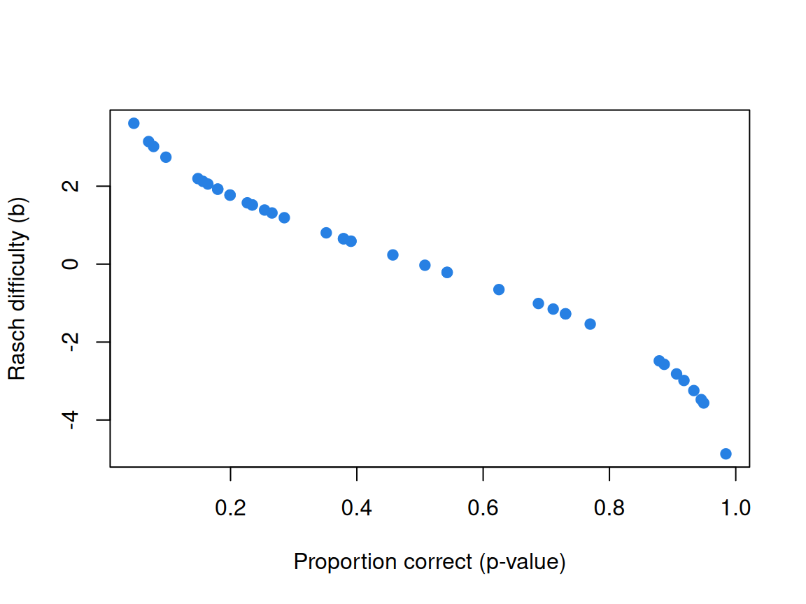
Code
sprintf("%.4f", cor(p, b, method = "spearman")) # rank correlation of p and b[1] "-0.9998"The rank correlation is −0.9998. That is sufficiency from the item side: with complete data an item’s total is sufficient for its difficulty (Mair & Hatzinger, 2007), and a few missing responses keep it from being exactly −1. The relationship is not linear, though: the Rasch scale stretches out the extremes, where a few percentage points correct correspond to a large difference in difficulty.
Code
theta <- fscores(m1)[, 1]
br <- seq(floor(min(c(theta, b))), ceiling(max(c(theta, b))), by = 0.25)
h <- hist(theta, breaks = br, plot = FALSE)
op <- par(mar = c(4, 4, 2, 1))
plot(NULL, xlim = c(-max(h$counts), 12), ylim = range(br), xaxt = "n",
     xlab = "", ylab = "Logits", main = "Wright map: chess_lnirt")
rect(-h$counts, h$breaks[-length(h$breaks)], 0, h$breaks[-1], col = "#dbeafe", border = "white")
points(rep(1.5, length(b)) + (seq_along(b) %% 8), b, pch = 18, col = "#c2410c")
abline(v = 0)
axis(1, at = c(-max(h$counts) / 2, 5), labels = c("People", "Items"), tick = FALSE)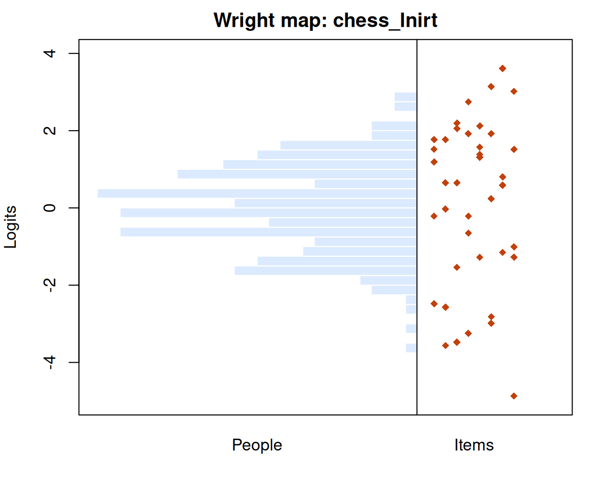
Code
par(op)
round(c(mean_theta = mean(theta), mean_b = mean(b)), 2)
mean_theta mean_b
0.00 0.12 Code
# mirt fixes the mean of the ability distribution at 0. Any other origin fits
# exactly as well: add 1 to every theta and every b, and no probability moves.
all.equal(plogis(outer(theta + 1, b + 1, "-")), plogis(outer(theta, b, "-")))
[1] TRUEThe mean ability is 0.00, the constraint mirt imposes, and adding 1 to every ability and difficulty leaves every probability unchanged (all.equal returns TRUE). So the mean difficulty says how hard the test is for this sample: 0.12, about a tenth of a logit, against an SD of ability of 1.22. The test is well targeted.
Does the model fit? One first look is the infit and outfit statistics (Wright & Masters, 1982): mean squared standardized residuals, which should be near 1 if the model is right. Values well below 1 mean an item is more predictable than the Rasch model expects (typically an item that discriminates better than average); values well above 1 mean it is noisier. How far from 1 is too far is the subject of Model fit and out-of-sample prediction.
Code
fit <- itemfit(m1, fit_stats = "infit")
head(fit[order(-abs(fit$z.outfit)), ], 5) # the five worst-fitting items, by |z|| item | outfit | z.outfit | infit | z.infit | |
|---|---|---|---|---|---|
| 9 | Y9 | 0.6360787 | -4.986545 | 0.7049058 | -5.7677088 |
| 8 | Y8 | 0.7291513 | -3.491464 | 0.7777831 | -4.1453249 |
| 38 | Y38 | 0.7295410 | -2.965869 | 0.8142504 | -3.2988899 |
| 10 | Y10 | 0.7308588 | -2.854375 | 0.8370314 | -2.8271237 |
| 15 | Y15 | 2.2221666 | 2.606262 | 1.1813203 | 0.9787916 |
Code
fit[which.max(fit$outfit), ] # the largest outfit of all 40 items| item | outfit | z.outfit | infit | z.infit | |
|---|---|---|---|---|---|
| 15 | Y15 | 2.222167 | 2.606262 | 1.18132 | 0.9787916 |
Code
# itemfit() computes residuals from mirt's default EAP abilities, which shrink toward
# the mean; method = "ML" uses maximum-likelihood abilities instead.
fit_ml <- itemfit(m1, fit_stats = "infit", method = "ML")
round(c(median_outfit_EAP = median(fit$outfit), median_outfit_ML = median(fit_ml$outfit)), 2)
median_outfit_EAP median_outfit_ML
0.95 1.01 Code
ml <- data.frame(item = fit_ml$item, outfit_ML = round(fit_ml$outfit, 2),
                 z_ML = round(fit_ml$z.outfit, 1))
ml[ml$item %in% c("Y8", "Y9", "Y10", "Y38"), ] # the four overfitting items above| item | outfit_ML | z_ML | |
|---|---|---|---|
| 8 | Y8 | 0.74 | -2.6 |
| 9 | Y9 | 0.63 | -4.0 |
| 10 | Y10 | 0.74 | -2.2 |
| 38 | Y38 | 0.74 | -2.3 |
Code
head(ml[order(-ml$outfit_ML), ], 3) # the largest outfits| item | outfit_ML | z_ML | |
|---|---|---|---|
| 2 | Y2 | 2.46 | 2.4 |
| 15 | Y15 | 2.45 | 2.8 |
| 33 | Y33 | 2.07 | 2.7 |
Code
itemfit(m1, empirical.plot = 15) # Y15: observed vs. model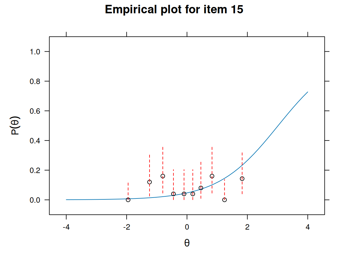
Four of the five worst-fitting items by \(|z|\) overfit (outfit from 0.64 to 0.73): they separate strong and weak players more sharply than a common slope allows. The exception is Y15, whose outfit of 2.2 is the largest of all 40 items under mirt’s default: by the size of its misfit, it is among the worst-fitting items on the test. It is the problem whose success barely moved with Elo in The likelihood and logistic regression. The empirical plot compares the model’s curve with the proportions solved among players grouped by ability. Those proportions barely rise: below-average players solve Y15 more often than the model expects, and the strongest group less often. Why is a question about the problem itself, which the responses alone can’t answer. These outfits come from mirt’s default EAP abilities, which pull outfit below 1 even when the model is true (Model fit and out-of-sample prediction). With maximum-likelihood abilities the median is 1.01 rather than 0.95, but the four overfitting items stay at 0.63 to 0.74, and Y15 (2.45) is second only to Y2 (2.46).
For contrast, a table whose job is to show a setting where one ability and equal slopes describe the data less well: wirs, six items from the 1990 Workplace Industrial Relations Survey analysed by Bartholomew (1998). Each item asks whether a kind of consultation took place about the most recent introduction of new equipment (1 = yes), from informal discussion with individual workers (item 1) through joint consultative committees (item 3) to paid union officials (wording from the ltm documentation, Rizopoulos, 2006). Because the sum score is sufficient, the Rasch model says what proportion of respondents with each sum score should say yes to each item, without estimating anyone’s \(\theta\) (the Go deeper callout gives the formula).
Code
wirs_url <- "https://redivis.com/api/v1/tables/datapages.item_response_warehouse:v57_0.wirs/rows?format=csv"
resp_w <- long2wide(read.csv(wirs_url))
dim(resp_w)
[1] 1005 6Code
m2 <- mirt(resp_w, 1, itemtype = "Rasch", verbose = FALSE)
b_w <- -coef(m2, simplify = TRUE)$items[, "d"]
# Because the sum score r is sufficient, the Rasch model predicts the proportion
# endorsing item i among respondents with sum score r without reference to theta:
#   P(x_i = 1 | r) = eps_i * gamma_(r-1)(items other than i) / gamma_r(all items),
# with eps = exp(-b) and gamma_r the elementary symmetric functions (see the
# Go deeper callout in the lesson).
esf <- function(eps) {               # gamma_0, gamma_1, ..., gamma_n
  g <- 1
  for (e in eps) g <- c(g, 0) + c(0, g) * e
  g
}
p_given_r <- function(b, i) {        # P(x_i = 1 | r) for r = 0, ..., n
  eps <- exp(-b); g <- esf(eps); g_i <- esf(eps[-i]); r <- seq_along(b)
  c(0, eps[i] * g_i[r] / g[r + 1])
}
r_w <- factor(rowSums(resp_w), levels = 0:6)
tab <- data.frame(r = 0:6, n = as.vector(table(r_w)),
  item1_observed = as.vector(tapply(resp_w[, 1], r_w, mean)),
  item1_rasch    = p_given_r(b_w, 1),
  item3_observed = as.vector(tapply(resp_w[, 3], r_w, mean)),
  item3_rasch    = p_given_r(b_w, 3))
round(tab, 2)| r | n | item1_observed | item1_rasch | item3_observed | item3_rasch |
|---|---|---|---|---|---|
| 0 | 132 | 0.00 | 0.00 | 0.00 | 0.00 |
| 1 | 284 | 0.23 | 0.17 | 0.04 | 0.11 |
| 2 | 256 | 0.56 | 0.38 | 0.19 | 0.26 |
| 3 | 191 | 0.58 | 0.59 | 0.52 | 0.44 |
| 4 | 89 | 0.36 | 0.76 | 0.81 | 0.65 |
| 5 | 50 | 0.40 | 0.90 | 0.96 | 0.84 |
| 6 | 3 | 1.00 | 1.00 | 1.00 | 1.00 |
Item 3 (a joint consultative committee) rises more steeply than the model allows: 0.04 of respondents with a sum score of 1 said yes, against a predicted 0.11, and 0.96 of those with 5, against 0.84. Item 1 (informal discussion with individual workers) barely tracks the sum score. It rises from 0.23 to 0.58 between sum scores 1 and 3, then falls to 0.36 and 0.40 at 4 and 5, where the model predicts 0.76 and 0.90. The data are telling us something about the construct: workplaces that use many formal channels don’t talk more with individual workers, so “amount of consultation” may not be a single dimension. Whether the Rasch model describes a dataset is something to check item by item, not assume (Model fit and out-of-sample prediction).
Problems
- The logit. Show that \(\frac{e^x}{1+e^x} = \frac{1}{1+e^{-x}}\). Then show that under the Rasch model, \(\log\frac{\Pr(x=1)}{\Pr(x=0)} = \theta - b\). What does a one-unit increase in \(\theta\) do to the odds of a correct response, on any item?
- Indeterminacy. Suppose \(\theta' = \theta + C\) and \(b' = b + C\). Show that \(\Pr(x = 1)\) is unchanged. Now suppose instead \(\theta' = k\theta\) and \(b' = kb\) for some \(k \ne 1\). Is the Rasch model still unchanged? What does your answer say about which feature of the scale the Rasch model does pin down, and how does it square with the difficulty pool’s chess SD of 1.75 against our 2.1?
- Specific objectivity in the chess data. By the Go deeper callout, among players who solved exactly one of problems \(i\) and \(k\), the proportion who solved \(i\) should be \(1/(1 + e^{b_i - b_k})\) whatever their ability. Pick two problems of middling difficulty, take the players who solved exactly one, and split them at the median of their sum score on the other 38. Compare the two halves with each other and with the prediction. Repeat for a pair that includes Y15. What do you see?
- Targeting. Draw the Wright map for
chess_lnirt. For which players does this test give the least information, and why? Suggest the difficulty of two items you would add to the test to improve measurement for them. - Fit, two ways. Using
itemfit(..., empirical.plot = i), compare several items inchess_lnirtand inwirs. Which dataset does the Rasch model describe better? Now run the simulation above withnp = 2000andni = 50and look at the same plots. What does “good fit” look like when you know the model is true? - Challenge: sufficiency in the data. In
chess_lnirt, find two players with the same sum score but very different response patterns. Compare their estimated abilities (fscores). Then fit a 2PL (itemtype = "2PL") and compare again. Explain what you see. Then the open part: if the 2PL fits the chess data better, how much would you lose by reporting the sum score anyway, and how would you decide?
Going further
- Rasch, G. (1960). Probabilistic models for some intelligence and attainment tests. Danish Institute for Educational Research; expanded edition, University of Chicago Press, 1980. https://openlibrary.org/works/OL4506215W. Where the model starts, including the case for separating people from items.
- Andersen, E. B. (1970). Asymptotic properties of conditional maximum-likelihood estimators. Journal of the Royal Statistical Society, Series B, 32(2), 283–301. https://doi.org/10.1111/j.2517-6161.1970.tb00842.x. Why conditioning on the sum score gives consistent difficulty estimates.
- Andersen, E. B. (1977). Sufficient statistics and latent trait models. Psychometrika, 42(1), 69–81. https://doi.org/10.1007/BF02293746. The converse: sufficiency of the sum score implies the Rasch model.
- Fischer, G. H. (1995). Derivations of the Rasch model. In G. H. Fischer & I. W. Molenaar (Eds.), Rasch models: Foundations, recent developments, and applications (pp. 15–38). Springer. https://doi.org/10.1007/978-1-4612-4230-7_2. The Go deeper callout, done properly and from several directions.
- Rasch, G. (1977). On specific objectivity: An attempt at formalizing the request for generality and validity of scientific statements. Danish Yearbook of Philosophy, 14, 58–94. https://doi.org/10.1163/24689300-01401006. Rasch’s own statement of specific objectivity.
- Wright, B. D. (1997). A history of social science measurement. Educational Measurement: Issues and Practice, 16(4), 33–45. https://doi.org/10.1111/j.1745-3992.1997.tb00606.x. The case for the Rasch model, from one of its leading advocates.
- Wright, B. D., & Masters, G. N. (1982). Rating scale analysis. MESA Press. https://www.rasch.org/rsa.htm. Infit and outfit, and Rasch analysis in practice.
- Tutz, G. (2025). A short guide to item response theory models. Springer. https://doi.org/10.1007/978-3-031-87271-6. Chapter 2 is a compact modern treatment of the binary Rasch model.
- Camilli, G. (1994). Origin of the scaling constant d = 1.7 in item response theory. Journal of Educational and Behavioral Statistics, 19(3), 293–295. https://doi.org/10.3102/10769986019003293. The 1.7 in the ICC challenge.
- Chalmers, R. P. (2012). mirt: A multidimensional item response theory package for the R environment. Journal of Statistical Software, 48(6). https://doi.org/10.18637/jss.v048.i06. The package used throughout.
- van der Maas, H. L. J., & Wagenmakers, E.-J. (2005). A psychometric analysis of chess expertise. American Journal of Psychology, 118(1), 29–60. https://doi.org/10.2307/30039042. The source of the chess data.
- Bartholomew, D. J. (1998). Scaling unobservable constructs in social science. Journal of the Royal Statistical Society, Series C, 47(1), 1–13. https://doi.org/10.1111/1467-9876.00094. The source of the
wirsdata. - From the IRW: simulating item difficulties shows what real difficulty distributions look like across the IRW (the baseline for the chess spread), and why they matter for simulation studies (Zhang, L., Liu, Y., Molenaar, D., Gilbert, J. B., Kanopka, K., & Domingue, B. W. (2025). Realistic simulation of item difficulties. PsyArXiv. https://doi.org/10.31234/osf.io/jbhxy_v4). The dimensionality, local dependence and 2PL discrimination vignettes take the model’s assumptions across the IRW.
- San Martín, E. (2017). Identification of item response theory models. In W. J. van der Linden (Ed.), Handbook of item response theory: Vol. 2. Statistical tools (pp. 127–150). Chapman and Hall/CRC. https://doi.org/10.1201/b19166-8. A handbook chapter on when the parameters of item response models are identified.
- von Davier, M. (2016). Rasch model. In W. J. van der Linden (Ed.), Handbook of item response theory: Vol. 1. Models (pp. 31–48). Chapman and Hall/CRC. https://doi.org/10.1201/9781315374512. A handbook chapter on the Rasch model.
Data sources
Data from the Item Response Warehouse (each table name links to its IRW page); references from IRW biblio.
chess_lnirt: Van Der Maas, H. L., & Wagenmakers, E. J. (2005). A psychometric analysis of chess expertise. The American journal of psychology, 118(1), 29-60. https://doi.org/10.2307/30039042. Licence: GPL-3.0.wirs: Bartholomew, D. (1998) Scaling unobservable constructs in social science. Applied Statistics, 47, 1–13. https://doi.org/10.1111/1467-9876.00094. Licence: GPL-3.0.
For instructors
- Source: EDUC 252 class 3 (slides c3, “Probabilistic item response modeling” through “Estimation of the RM”) and the code in
ben-domingue/252:c3/rasch0.R,c3/rasch1.R,c3/rasch2.R. - Timing: the core ideas and widgets fit in about 75 minutes of class; the real-data section works well as an in-class lab. The Go deeper callout is optional reading for students with some mathematical statistics.
- Changed from 252 (retrofit, 09-24): the sufficiency derivation (factorization, conditional ML, specific objectivity as a theorem, Andersen’s converse) was added as a Go deeper callout; the
wirscontrast now compares observed and model-implied proportions given the sum score rather than an empirical plot; the “wide spread” of chess difficulties is judged against the IRW difficulty pool; a problem on readingmirt’s rawdwas replaced by problem 3 (specific objectivity in the chess data). - Held back: item and test information, and the estimation algorithms, have their own lessons. The problem set questions on Rasch fit statistics (outfit’s sampling distribution) are in Model fit and out-of-sample prediction.
- Solutions: held back in
solutions/rasch.qmd(not published).