From the 1PL to the 4PL
What this is for
The Rasch model gives every item the same slope, and the chess data have already turned up an item that doesn’t go along: problem Y15, about as hard as Y29, whose success barely moves with skill. What happens when each item gets its own slope, and then its own floor and ceiling? This lesson builds that family, from the 1PL to the 4PL, asks what each new parameter costs and what the data can say about it, and fits all four to the Reading the Mind in the Eyes Test. On that test the evidence here points to the 2PL, and most of the lesson is that evidence.
Goals
By the end of this lesson you should be able to:
- write down the 4PL, say what \(a\), \(b\), \(c\) and \(u\) do to a curve, and which constraints give the 3PL, 2PL and Rasch model;
- explain why the weighted score \(\sum_i a_i x_i\) replaces the sum score under the 2PL, and why crossing curves give up specific objectivity;
- convert
mirt’s intercept to a difficulty, and say how each model fixes the unit of the scale; - explain why a lower asymptote is hard to estimate, and what data would let one be estimated;
- fit all four models with
mirtand compare them by BIC and by what they say about respondents.
Core ideas
One family of curves
One formula covers every model here. For person \(j\) and item \(i\), \[\Pr(x_{ij} = 1) = c_i + (u_i - c_i)\,\frac{\exp\big(a_i(\theta_j - b_i)\big)}{1 + \exp\big(a_i(\theta_j - b_i)\big)}.\]
- \(b_i\) is the item’s difficulty, its location on the \(\theta\) scale.
- \(a_i\) is its slope or discrimination: how quickly the probability rises as \(\theta\) passes \(b_i\).
- \(c_i\) is the lower asymptote, the probability of success at very low ability; on multiple-choice items it is called the guessing parameter.
- \(u_i\) is the upper asymptote; below 1, even the strongest respondents sometimes miss (a “slip”).
“PL” stands for “parameter logistic”, and the number counts the free item parameters. The Rasch model, a 1PL, frees only \(b\) (\(a = 1\), \(c = 0\), \(u = 1\)). The 2PL frees \(a\) and the 3PL frees \(c\) as well, both from Birnbaum’s chapters in Lord & Novick (1968). The 4PL frees \(u\) too (Barton & Lord, 1981; Loken & Rulison, 2010).
Try it: four parameters
Move \(a\) and the curve pivots around \(b\); near zero it is almost flat. Raising \(c\) lifts the floor, and lowering \(u\) (the last slider) drops the ceiling. The point at \(\theta = b\) always sits halfway between the asymptotes, so once \(c > 0\) or \(u < 1\), difficulty no longer means “the ability at which the probability is 0.5”.
Four items, with different values of all four parameters:
What slopes cost: sufficiency and crossing curves
What takes the sum score’s place under the 2PL? Write out one person’s likelihood, as the Rasch lesson’s Go deeper callout did: \[\Pr(\mathbf{x} \mid \theta) = \prod_i \frac{\exp\big(x_i a_i(\theta - b_i)\big)}{1 + \exp\big(a_i(\theta - b_i)\big)} = \frac{\exp\big(\theta \sum_i a_i x_i\big)\,\exp\big(-\sum_i a_i b_i x_i\big)}{\prod_i \big(1 + \exp(a_i(\theta - b_i))\big)}.\] The data meet \(\theta\) only through the weighted score \(\sum_i a_i x_i\), so under the 2PL it is sufficient (Birnbaum, 1968). A correct answer counts in proportion to its item’s slope. The weights are estimated item parameters, though; Andersen (1977) showed that a sufficient statistic free of the item parameters exists only under the Rasch model. Under the 3PL the lower asymptote spoils the factorization, and no simple statistic is sufficient.
Reading mirt, and what fixes the scale
mirt (Chalmers, 2012) writes these models with an intercept, \(\Pr(x = 1) = g + (u - g)\,\text{logit}^{-1}(a\theta + d)\); its g is our \(c\) and its u is our \(u\). Matching \(a\theta + d\) with \(a(\theta - b)\) gives \(b = -d/a\), the conversion every chunk below uses. When \(a\) is near 0, that ratio can be enormous, as the chess data will show.
What fixes the unit of \(\theta\)? The model only sees \(a(\theta - b)\), so multiplying every \(\theta\) and \(b\) by \(k\) and dividing every \(a\) by \(k\) changes no probability. The unit is a convention the software sets, as the origin was (The Rasch model): the Rasch fit fixes the slopes at 1 and estimates the SD of \(\theta\); the 2PL fixes that SD at 1. A Rasch fit and a 1PL with one common, estimated slope are then the same model reporting different \(a\) and \(b\). That matters when reading output or comparing numbers across fits, the problem Linking and equating takes up, but it says nothing about the data.
What the lower asymptote needs
The lower asymptote describes people far below an item’s difficulty. If few respondents are down there, the data say little about it, and a 2PL, with a lower slope and a shifted difficulty, can imitate a 3PL where the respondents are.
Try it: can a 2PL stand in for a 3PL?
As the widget loads, mean ability is 1.5, so the item is easy for most respondents. The curves differ by at most about 0.01 where respondents are, parting only to the left, where almost nobody is. Slide the mean ability down to −2 and the largest difference grows eight-fold, to 0.08: now many respondents sit near the floor, and the floor matters.
Domingue et al. (2024) looked at this through prediction. They simulated data from the 3PL and asked how much better a fitted 3PL predicted new responses than a fitted 2PL, using the IMV, a measure of predictive gain that Model fit and out-of-sample prediction teaches. The average gain never exceeded 0.001, even with pronounced guessing in the generating model, and across 89 IRW datasets it averaged 0.00016. They connect this to the difficulty of identifying the 3PL’s parameters (Maris & Bechger, 2009; Haberman, 2005; von Davier, 2009), noting that 3PL estimates may still flag items with guessing problems. The data have more to say about \(c\) when the items are multiple choice and a good share of respondents sits near chance, when the sample is large, or when \(c\) is fixed or given a prior, as in Guessing and priors; whether the 3PL then predicts held-out responses better is a comparison the data can make.
The upper asymptote: ceilings and slips
What does \(u < 1\) mean? That respondents far above an item’s difficulty still sometimes miss it: through carelessness, a slip, or an item harder than it looks for experts. Barton and Lord (1981) added the upper asymptote to the 3PL in an ETS report; Loken and Rulison (2010) estimated the 4PL with Bayesian methods and applied it to a delinquency scale.
The ceiling mirrors the floor: estimating \(u\) needs many respondents far above the item, missing it now and then. Most data have few, so \(u\) is weakly identified. On the RMET, the 4PL had not converged when EM stopped at its 500-cycle limit (below).
The same two asymptotes return, without a curve between them, in cognitive diagnosis. In the DINA model (Junker & Sijtsma, 2001), a respondent who has every attribute an item requires answers correctly with probability \(1 - s\), where \(s\) is the item’s slip parameter, and a respondent who lacks any of them with probability \(g\), its guess. Cognitive diagnostic models, an extension lesson, takes this up.
Two philosophies
The choice between these models is also a choice between two traditions, which Andrich (2004) describes as incompatible paradigms in Kuhn’s sense. What does each assume?
- The model comes first. The Rasch tradition starts from what measurement should mean: a sufficient sum score, and comparisons that don’t depend on which items or people were used (Rasch, 1960; Wright, 1997). It assumes items can be revised until they fit, and treats misfit as information about the items. It suits building an instrument you can still change.
- The data come first. The tradition that runs from Birnbaum through Lord (1980) takes the items as given and adds parameters until the curves describe them, accepting weighted scores and crossing curves. It suits analysing a test you can’t change.
Some of the disagreement is about values, which data can’t settle; some is empirical, and the RMET tests it below.
Beyond four: asymmetric curves
All four models give point-symmetric curves. Samejima (2000) proposed the logistic positive exponent family, which raises a logistic curve to a positive power so that it can rise slowly and then steeply, or the reverse. Lee and Bolt (2018) study what asymmetry can say about item complexity, and the IRW’s asymmetric models vignette fits such models across its tables.
Simulate
The code below simulates 1,000 respondents answering 20 items from a 3PL with \(c = 0.25\) on every item, then fits the Rasch model, the 2PL and the 3PL. It runs in your browser; the first run takes 20–30 seconds while R and mirt load, and the fits a little longer.
With the seed as written, the estimates of \(c\) have a median of 0.25, right on the truth, but range from 0 to 0.48. BIC prefers the Rasch model (25,347, against 25,362 for the 2PL and 25,464 for the 3PL), although the 3PL generated the data. The three models’ abilities correlate 0.97 to 0.99 with each other.
Now change np. At 300, the median estimate of \(c\) drops to 0.06. At 10,000 (run that in your own R session), the estimates range from 0.07 to 0.42, BIC finally prefers the 3PL, and the abilities still correlate 0.99 or above. The lower asymptote needs a lot of data to settle; the abilities hardly notice it either way.
Download this code to run it in your own R session.
With real data
Our main example is wilmer-rmet-normative-data-set-2022, responses to the Reading the Mind in the Eyes Test (RMET; Baron-Cohen et al., 2001), a measure of reading mental states from the eye region of a face. Each of its 36 items offers four words, one of them correct. The data are the normative sample Kim et al. (2024) released with their Multiracial RMET (the landing page describes the newer test; this table holds the original). Its job is to be a test where the lower asymptote has an obvious prediction: with four options, chance is 0.25. A response is 1 when the respondent chose the correct word. Download the code to run every chunk yourself.
Code
library(mirt)
# Each IRW table has a landing page (itemresponsewarehouse.org/tables/<name>/)
# with a CSV download. This link is pinned to one version of the data.
rmet_url <- "https://redivis.com/api/v1/tables/datapages.item_response_warehouse_2:v22_0.wilmer-rmet-normative-data-set-2022/rows?format=csv"
df <- read.csv(rmet_url)
# resp is 1 when the respondent chose the correct word of the four; resp_raw is the
# word they chose. Every respondent answered every item once, and there are no waves.
head(df[, c("id", "item", "resp", "resp_raw")], 3)| id | item | resp | resp_raw |
|---|---|---|---|
| 41 | item_28 | 0 | affectionate |
| 41 | item_8 | 1 | despondent |
| 41 | item_25 | 1 | interested |
Code
c(respondents = length(unique(df$id)), items = length(unique(df$item)),
  responses_per_respondent = unique(as.vector(table(df$id))),
  words_offered_per_item = unique(as.vector(tapply(df$resp_raw, df$item, function(x) length(unique(x))))))
respondents items responses_per_respondent
17680 36 36
words_offered_per_item
4 Code
# IRW tables are long (one row per response); mirt wants wide (one row per respondent).
long2wide <- function(df) {
  wide <- tapply(df$resp, list(df$id, df$item), function(x) x[1])
  as.data.frame(wide[, order(as.numeric(gsub("\\D", "", colnames(wide))))])
}
resp <- long2wide(df)
p <- colMeans(resp)
round(range(p), 2)     # proportion correct: the easiest and hardest items
[1] 0.56 0.86All 17,680 respondents answered all 36 items. The items are easy for this sample: 56% to 86% chose the correct word.
Code
# Four models, from the Rasch model to the 4PL. To keep the fits to a minute or two
# we use a random 5,000 of the 17,680 respondents.
set.seed(252)
rs <- resp[sample(nrow(resp), 5000), ]
models <- c("Rasch", "2PL", "3PL", "4PL")
fits <- lapply(setNames(models, models), function(m) mirt(rs, 1, itemtype = m, verbose = FALSE))
data.frame(parameters = sapply(fits, extract.mirt, "nest"),
           BIC = round(sapply(fits, extract.mirt, "BIC")),
converged = sapply(fits, extract.mirt, "converged"))| parameters | BIC | converged | |
|---|---|---|---|
| Rasch | 37 | 205192 | TRUE |
| 2PL | 72 | 204337 | TRUE |
| 3PL | 108 | 204617 | TRUE |
| 4PL | 144 | 204707 | FALSE |
BIC (Schwarz, 1978) adds a penalty for each parameter to minus twice the log likelihood; smaller is better. It prefers the 2PL (204,337) to the Rasch model (205,192, or 855 higher), the 3PL (204,617) and the 4PL (204,707). The 4PL hadn’t converged at EM’s 500-cycle limit, itself a sign that the data say little about four parameters per item. BIC says whether a model is preferred, not how much it improves predictions of new responses; that is for Model fit and out-of-sample prediction.
Code
# The 4PL's upper asymptotes (mirt's u, our u), and how many respondents are up
# where a ceiling would show: 34 or more of 36 correct.
u_hat <- coef(fits$`4PL`, simplify = TRUE)$items[, "u"]
round(quantile(u_hat, c(0, 0.25, 0.5, 0.75, 1)), 2)
0% 25% 50% 75% 100%
0.71 0.85 0.96 0.99 1.00 Code
c(at_or_above_34 = sum(rowSums(resp) >= 34), share = round(mean(rowSums(resp) >= 34), 3))at_or_above_34 share
352.00 0.02 The 4PL’s ceilings run from 0.71 to 1.00 (median 0.96), yet only 2% of respondents answered 34 or more items correctly: like the floors, they rest on few respondents.
Code
# mirt writes the 2PL as a*theta + d. In our notation the difficulty is b = -d/a.
cf2 <- coef(fits$`2PL`, simplify = TRUE)$items
a <- cf2[, "a1"]
b <- -cf2[, "d"] / a
round(c(min_a = min(a), median_a = median(a), max_a = max(a)), 2)
min_a median_a max_a
0.19 0.67 1.13 Code
round(c(min_b = min(b), max_b = max(b)), 2)min_b max_b
-3.23 -0.39 Code
# The spread of the slopes on the log scale (0 under the Rasch model), and the ratio
# of the 90th to the 10th percentile. "Across the IRW" puts these in context.
round(c(sd_log_a = sd(log(a)), ratio_90_10 = unname(quantile(a, 0.9) / quantile(a, 0.1))), 2)
sd_log_a ratio_90_10
0.42 2.81 The slopes run from 0.19 to 1.13, a ratio of about 6 (\(1.13/0.19 \approx 5.9\)). Every difficulty is negative (−3.23 to −0.39): each item is easy for an average respondent. On the log scale the slopes have an SD of 0.42, which Across the IRW compares with the rest of the warehouse.
Code
# mirt calls the lower asymptote g; it is our c.
c_hat <- coef(fits$`3PL`, simplify = TRUE)$items[, "g"]
round(quantile(c_hat, c(0, 0.25, 0.5, 0.75, 1)), 2)
0% 25% 50% 75% 100%
0.00 0.00 0.01 0.16 0.57 Code
# How many respondents are down where the lower asymptote lives? Chance on 36
# four-option items is 9 correct.
r <- rowSums(resp)
c(at_or_below_9 = sum(r <= 9), share = round(mean(r <= 9), 4), median_sum_score = median(r))
at_or_below_9 share median_sum_score
84.0000 0.0048 26.0000 The median estimate of \(c\) is 0.01. Why so far from 0.25? Only 84 of the 17,680 respondents (0.48%) answered 9 or fewer items correctly, the score expected from picking words at random; the median respondent answered 26. The lower asymptote describes people almost absent from these data. This says not that RMET respondents never guess, but that these data can’t tell how often. Which wrong words they chose is a question for Nominal response and multiple-choice models, with the same data.
Code
# Ability estimates (EAP) from the four models, for the same 5,000 respondents.
theta <- sapply(fits, function(m) fscores(m)[, 1])
round(cor(theta), 3)
Rasch 2PL 3PL 4PL
Rasch 1.000 0.983 0.982 0.972
2PL 0.983 1.000 0.999 0.987
3PL 0.982 0.999 1.000 0.990
4PL 0.972 0.987 0.990 1.000The four models’ abilities correlate from 0.972 to 0.999, and the three with free slopes at 0.987 or above. The choice matters little for ranking respondents, more for what we say about items.
What does the evidence say about the RMET? The slopes differ six-fold, BIC prefers the 2PL to the Rasch model by 855 points, the lower asymptote can’t be estimated from a sample with almost no one near chance, and the richer models’ abilities correlate with the 2PL’s at 0.987 or above. On this evidence the 2PL describes the test as it stands; how much better it predicts held-out responses is the comparison Model fit and out-of-sample prediction makes. If the RMET were being revised, the Rasch tradition’s question (which items to rewrite so that one slope fits them all) would be a fair one.
Chess, again
Our contrast table is chess_lnirt, the Amsterdam Chess Test (van der Maas & Wagenmakers, 2005), used again on purpose to show what the 2PL makes of Y15 (three players with no responses dropped, as before).
Code
chess_url <- "https://redivis.com/api/v1/tables/datapages.item_response_warehouse:v57_0.chess_lnirt/rows?format=csv"
chess <- long2wide(read.csv(chess_url))
chess <- chess[rowSums(!is.na(chess)) > 0, ]   # three players have no responses
dim(chess)
[1] 256 40Code
m_r <- mirt(chess, 1, itemtype = "Rasch", verbose = FALSE)
m_2 <- mirt(chess, 1, itemtype = "2PL", verbose = FALSE)
cc <- coef(m_2, simplify = TRUE)$items
a_ch <- cc[, "a1"]
b_ch <- -cc[, "d"] / a_ch                     # b = -d/a
round(sort(a_ch)[c(1:3, 38:40)], 2)          # the flattest and steepest items
Y15 Y27 Y36 Y9 Y26 Y29
0.02 0.35 0.47 2.91 3.19 3.79 Code
round(rbind(a = a_ch, b = b_ch)[, c("Y15", "Y29")], 2) Y15 Y29
a 0.02 3.79
b 136.52 1.56Code
round(c(BIC_Rasch = extract.mirt(m_r, "BIC"), BIC_2PL = extract.mirt(m_2, "BIC")))BIC_Rasch BIC_2PL
8960 8906 The 2PL slopes run from 0.02 (Y15) to 3.79 (Y29), and BIC prefers the 2PL to the Rasch model (8,906 against 8,960). Y15’s curve is nearly flat: a player’s ability tells us almost nothing about whether they solve it. Its difficulty of 136.52 comes from dividing by a slope near zero; for an item this flat, \(b\) has no useful meaning.
Code
# The 2PL curves for Y15 and Y29, with the proportion solving each item among
# players grouped by their sum score on the other 38 items (thirds).
rest <- rowSums(chess[, setdiff(names(chess), c("Y15", "Y29"))], na.rm = TRUE)
grp <- cut(rest, quantile(rest, 0:3 / 3), include.lowest = TRUE,
           labels = c("bottom third", "middle third", "top third"))
obs <- sapply(chess[, c("Y15", "Y29")], function(x) tapply(x, grp, mean, na.rm = TRUE))
cbind(players = table(grp), round(obs, 2))
players Y15 Y29
bottom third 89 0.09 0.00
middle third 83 0.05 0.02
top third 84 0.10 0.19Code
th_grp <- tapply(fscores(m_2)[, 1], grp, mean)   # mean 2PL ability in each group
th <- seq(-3, 3, length.out = 200)
icc <- function(i) plogis(a_ch[i] * (th - b_ch[i]))
op <- par(mar = c(4, 4, 1, 1))
plot(th, icc("Y29"), type = "l", lwd = 2, col = "#2780e3", ylim = c(0, 1),
     xlab = "Ability (2PL scale)", ylab = "P(solved)")
lines(th, icc("Y15"), lwd = 2, col = "#c2410c")
points(th_grp, obs[, "Y29"], pch = 19, col = "#2780e3")
points(th_grp, obs[, "Y15"], pch = 17, col = "#c2410c")
legend("topleft", c("Y29", "Y15"), col = c("#2780e3", "#c2410c"), lwd = 2, pch = c(19, 17), bty = "n")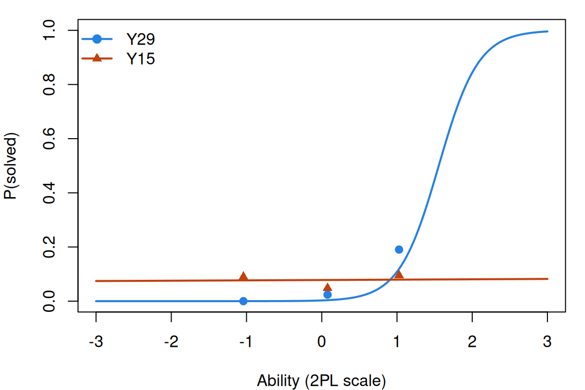
Code
par(op)
# Where the two curves cross: a29 (theta - b29) = a15 (theta - b15).
cross <- (a_ch["Y29"] * b_ch["Y29"] - a_ch["Y15"] * b_ch["Y15"]) / (a_ch["Y29"] - a_ch["Y15"])
round(c(crossing_theta = unname(cross), share_of_players_below = mean(fscores(m_2)[, 1] < cross)), 2)
crossing_theta share_of_players_below
0.91 0.82 The curves cross at \(\theta = 0.91\); for the 82% of players below it Y15 is the easier problem, and for the strongest, Y29. The grouped proportions (points) agree without the model: in the bottom third of players (by score on the other 38 problems) 9% solved Y15 and none Y29; in the top third, 10% and 19%. “Y15 is easier than Y29” is true for some players and false for others: specific objectivity given up, in data.
Code
# Under the Rasch model, players with the same sum score get the same ability
# estimate. Under the 2PL, the weighted score sum(a_i x_i) takes its place.
th_r <- fscores(m_r)[, 1]
th_2 <- fscores(m_2)[, 1]
sum_score <- rowSums(chess, na.rm = TRUE)
complete <- rowSums(is.na(chess)) == 0        # the sum score compares only on complete rows
spread <- function(th) tapply(th[complete], sum_score[complete], function(x) diff(range(x)))
round(c(max_spread_Rasch = max(spread(th_r)), max_spread_2PL = max(spread(th_2))), 2)
max_spread_Rasch max_spread_2PL
0.00 0.63 Code
# The players with a sum score of 20 (complete responses only), under both models.
s20 <- complete & sum_score == 20
tab20 <- data.frame(theta_Rasch = th_r[s20], theta_2PL = th_2[s20],
                    weighted_score = as.vector(as.matrix(chess[s20, ]) %*% a_ch))
round(tab20[order(tab20$weighted_score), ], 2)| theta_Rasch | theta_2PL | weighted_score | |
|---|---|---|---|
| 13 | 0.29 | 0.06 | 22.29 |
| 8 | 0.29 | 0.14 | 23.31 |
| 12 | 0.29 | 0.18 | 23.75 |
| 3 | 0.29 | 0.22 | 24.35 |
| 15 | 0.29 | 0.26 | 24.81 |
| 6 | 0.29 | 0.27 | 24.93 |
| 1 | 0.29 | 0.28 | 25.12 |
| 9 | 0.29 | 0.30 | 25.45 |
| 14 | 0.29 | 0.31 | 25.59 |
| 2 | 0.29 | 0.32 | 25.67 |
| 7 | 0.29 | 0.33 | 25.74 |
| 4 | 0.29 | 0.35 | 26.08 |
| 10 | 0.29 | 0.35 | 26.14 |
| 11 | 0.29 | 0.38 | 26.44 |
| 5 | 0.29 | 0.39 | 26.65 |
Among players with complete responses, the Rasch model gives everyone with the same sum score the same estimate (largest spread 0.00); the 2PL spreads them by up to 0.63. The fifteen players who solved exactly 20 problems share one Rasch estimate, 0.29, but get 2PL estimates from 0.06 to 0.39, in the order of their weighted scores.
Code
# The Rasch fit fixes every slope at 1 and estimates the SD of ability. A "1PL"
# with one common slope fixes the SD at 1 and estimates the slope instead: the same
# model in another unit, so its slope equals the Rasch SD of ability.
m_1 <- mirt(chess, mirt.model("F = 1-40\nCONSTRAIN = (1-40, a1)"), itemtype = "2PL", verbose = FALSE)
round(c(SD_theta_Rasch = sqrt(coef(m_r, simplify = TRUE)$cov[1, 1]),
        common_slope_1PL = coef(m_1, simplify = TRUE)$items[1, "a1"]), 2)
SD_theta_Rasch common_slope_1PL
1.22 1.22 Last, the units point: a 1PL with one common slope reports that slope as 1.22, the Rasch fit’s SD of ability.
Problems
- Weighted scores. Show that under the 2PL, \(\sum_i a_i x_i\) is sufficient for \(\theta\). Then, for the 3PL, find two patterns on three items of your choosing with the same \(\sum_i a_i x_i\) but different maximum-likelihood estimates.
- What \(b\) means now. For the 3PL, show that at \(\theta = b\) the probability is \((1 + c)/2\). At what \(\theta\) is the probability 0.5? What does \(b\) describe, in words, once \(c > 0\)? And for the 4PL?
- Where the floor is. Fit the 2PL and the 3PL to the RMET using only the respondents in the bottom quarter of sum scores. Do the estimated lower asymptotes change? Explain what you see, and why selecting on the same items’ sum score might itself cause trouble.
- Reading \(c\). A colleague wants to report the RMET’s 3PL lower asymptotes as “the rate at which people guess on each item”. What would you tell them, using this lesson’s output?
- Crossing curves. In the chess data, find two problems other than Y15 whose 2PL curves cross where most players sit. For which players is each the easier one? Check against grouped proportions, as the lesson did for Y15 and Y29.
- Challenge: when does the model matter? The four models’ RMET abilities correlate at 0.97 or above. When would the choice still matter for a decision about one person? Think about the ends of the scale, cut scores and unusual patterns; Loken & Rulison (2010) is one place to start. This one is open: I don’t know of a general answer.
Across the IRW
How much do slopes vary in real data? For each dichotomous IRW table with at least 250 respondents, 5 to 200 items and a nearly complete response matrix, compute.R fits the Rasch model and the 2PL and summarises the slopes’ spread by the SD of \(\log a\), which rescaling \(\theta\) leaves alone. It is 0 under the Rasch model, and 0.42 for the RMET above (0.43 in the corpus run’s own sample).
Code
dd_path <- file.path("..", "deepdives", "1pl-to-4pl", "results.rds")
dd <- if (file.exists(dd_path)) readRDS(dd_path) else NULL
if (!is.null(dd)) {
  s <- dd$summary[order(dd$summary$sd_log_a), ]
  print(data.frame(table = s$table, items = s$n_items, respondents = s$n_resp,
                   sd_log_a = round(s$sd_log_a, 2), ratio_90_10 = round(s$ratio_90_10, 1),
                   BIC_prefers_2PL = s$prefers_2pl, converged = s$converged), row.names = FALSE)
  op <- par(mar = c(4, 1, 1, 1))
  known <- s$table %in% c("chess_lnirt", "wilmer-rmet-normative-data-set-2022")
  plot(s$sd_log_a, rep(0, nrow(s)), pch = 19, cex = 1.3, yaxt = "n", ylab = "", bty = "n",
       col = ifelse(known, "#c2410c", "#2780e3"), xlim = c(0, max(1.5, s$sd_log_a, na.rm = TRUE)),
       xlab = "SD of log slope within a table (0 = Rasch)")
  abline(v = 0, lty = 2, col = "#999")
  par(op)
}
table items respondents sd_log_a ratio_90_10
paraguay_2021_women_family 20 3276 0.28 1.8
peters_2025_si_current 6 5000 0.39 2.2
wilmer-rmet-normative-data-set-2022 36 5000 0.43 2.9
chess_lnirt 40 256 0.87 4.0
taylorabdulai_2025_incentives 7 377 1.26 10.4
chuemchit_2024_nonpartner_violence 5 494 1.42 14.3
BIC_prefers_2PL converged
TRUE TRUE
TRUE TRUE
TRUE TRUE
TRUE TRUE
TRUE TRUE
FALSE FALSE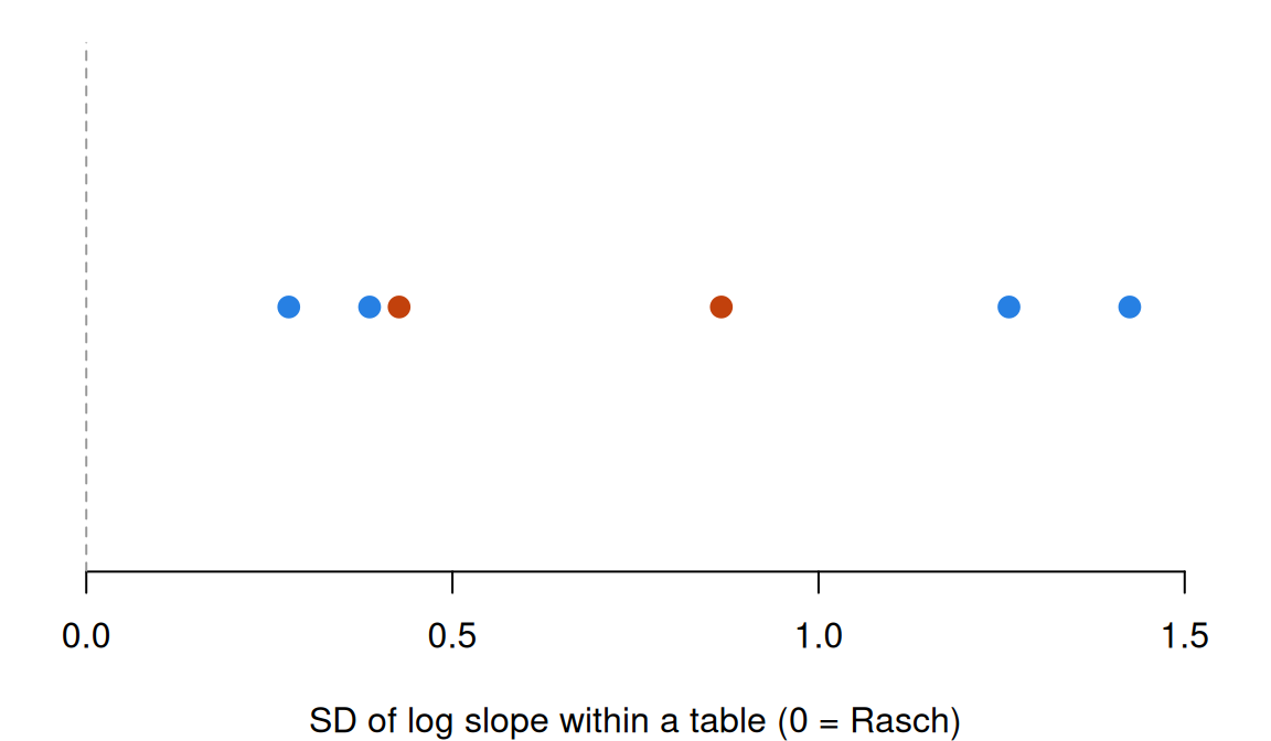
Run on 24 September 2026: 6 tables fitted, 0 failed. In 5 of the 6, BIC prefers the 2PL to the Rasch model. The SD of log slopes runs from 0.28 to 1.42 (median 0.65); chess and the RMET are marked in orange.
This answers the Rasch lesson’s question: are equal slopes plausible? The nearer a table’s SD of \(\log a\) is to 0, the more so. The IRW’s 2PL discrimination vignette takes the question to its cognitive tables, slope by slope. Whether the extra parameters improve predictions of new responses is the other half, reported in Model fit and out-of-sample prediction.
Going further
- Lord, F. M., & Novick, M. R. (1968). Statistical theories of mental test scores (with contributions by A. Birnbaum). Addison-Wesley. https://openlibrary.org/works/OL6568286W. Birnbaum’s chapters 17–20 introduce the logistic 2PL and 3PL.
- Lord, F. M. (1980). Applications of item response theory to practical testing problems. Erlbaum. https://doi.org/10.4324/9780203056615. The 3PL at work on real tests.
- Barton, M. A., & Lord, F. M. (1981). An upper asymptote for the three-parameter logistic item-response model. ETS Research Report Series, 1981(1). https://doi.org/10.1002/j.2333-8504.1981.tb01255.x. Where the fourth parameter starts.
- Loken, E., & Rulison, K. L. (2010). Estimation of a four-parameter item response theory model. British Journal of Mathematical and Statistical Psychology, 63(3), 509–525. https://doi.org/10.1348/000711009x474502. A Bayesian 4PL, and what simpler models miss at the ends of the scale.
- Andersen, E. B. (1977). Sufficient statistics and latent trait models. Psychometrika, 42(1), 69–81. https://doi.org/10.1007/BF02293746. Why only the Rasch model has a sufficient statistic free of item parameters.
- Domingue, B. W., Kanopka, K., Kapoor, R., Pohl, S., Chalmers, R. P., Rahal, C., & Rhemtulla, M. (2024). The InterModel Vigorish as a lens for understanding (and quantifying) the value of item response models for dichotomously coded items. Psychometrika, 89(3), 1034–1054. https://doi.org/10.1007/s11336-024-09977-2. How much the 2PL and 3PL add to prediction, in simulation and across IRW datasets.
- Maris, G., & Bechger, T. (2009). On interpreting the model parameters for the three parameter logistic model. Measurement: Interdisciplinary Research and Perspectives, 7(2), 75–88. https://doi.org/10.1080/15366360903070385. What the 3PL’s parameters can and can’t be read as.
- von Davier, M. (2009). Is there need for the 3PL model? Guess what? Measurement: Interdisciplinary Research and Perspectives, 7(2), 110–114. https://doi.org/10.1080/15366360903117079. A commentary in the same issue.
- Haberman, S. J. (2005). Identifiability of parameters in item response models with unconstrained ability distributions. ETS Research Report Series, 2005(2), i–22. https://doi.org/10.1002/j.2333-8504.2005.tb02001.x. The identification question in general form.
- Andrich, D. (2004). Controversy and the Rasch model: A characteristic of incompatible paradigms? Medical Care, 42(1 Suppl.), I-7–I-16. https://doi.org/10.1097/01.mlr.0000103528.48582.7c. The two traditions, set out side by side.
- Wright, B. D. (1997). A history of social science measurement. Educational Measurement: Issues and Practice, 16(4), 33–45. https://doi.org/10.1111/j.1745-3992.1997.tb00606.x. The case for choosing items that fit the Rasch model.
- Samejima, F. (2000). Logistic positive exponent family of models: Virtue of asymmetric item characteristic curves. Psychometrika, 65(3), 319–335. https://doi.org/10.1007/BF02296149. Curves that aren’t symmetric.
- Lee, S., & Bolt, D. M. (2018). Asymmetric item characteristic curves and item complexity: Insights from simulation and real data analyses. Psychometrika, 83(2), 453–475. https://doi.org/10.1007/s11336-017-9586-5. What asymmetry might say about items.
- Schwarz, G. (1978). Estimating the dimension of a model. The Annals of Statistics, 6(2), 461–464. https://doi.org/10.1214/aos/1176344136. The BIC.
- Chalmers, R. P. (2012). mirt: A multidimensional item response theory package for the R environment. Journal of Statistical Software, 48(6). https://doi.org/10.18637/jss.v048.i06. The package, including its intercept parameterization.
- Baron-Cohen, S., Wheelwright, S., Hill, J., Raste, Y., & Plumb, I. (2001). The “Reading the Mind in the Eyes” Test revised version: A study with normal adults, and adults with Asperger syndrome or high-functioning autism. Journal of Child Psychology and Psychiatry, 42(2), 241–251. https://doi.org/10.1111/1469-7610.00715. The source of the RMET.
- Kim, H. A., Kaduthodil, J., Strong, R. W., Germine, L. T., Cohan, S., & Wilmer, J. B. (2024). Multiracial Reading the Mind in the Eyes Test (MRMET): An inclusive version of an influential measure. Behavior Research Methods, 56(6), 5900–5917. https://doi.org/10.3758/s13428-023-02323-x. The source of the RMET data.
- van der Maas, H. L. J., & Wagenmakers, E.-J. (2005). A psychometric analysis of chess expertise. American Journal of Psychology, 118(1), 29–60. https://doi.org/10.2307/30039042. The source of the chess data.
- From the IRW: the 2PL discrimination vignette (slopes across its cognitive tables) and the asymmetric models vignette.
- van der Linden, W. J. (2016). Unidimensional logistic response models. In W. J. van der Linden (Ed.), Handbook of item response theory: Vol. 1. Models (pp. 13–30). Chapman and Hall/CRC. https://doi.org/10.1201/9781315374512. A handbook chapter on the one-, two- and three-parameter logistic models.
Data sources
Data from the Item Response Warehouse (each table name links to its IRW page); references from IRW biblio.
wilmer-rmet-normative-data-set-2022: Kim, H.A., Kaduthodil, J., Strong, R.W. et al. Multiracial Reading the Mind in the Eyes Test (MRMET): An inclusive version of an influential measure. Behav Res 56, 5900–5917 (2024). https://doi.org/10.3758/s13428-023-02323-x. Licence: CC BY 4.0.chess_lnirt: Van Der Maas, H. L., & Wagenmakers, E. J. (2005). A psychometric analysis of chess expertise. The American journal of psychology, 118(1), 29-60. https://doi.org/10.2307/30039042. Licence: GPL-3.0.
For instructors
- Source: EDUC 252 class 4 (slides c4, 18–34 and 60–61) and the code in
ben-domingue/252:c4/enem1.R,c4/enem2.R,c4/enem3.R. - Timing: the core ideas and widgets take about 60 minutes; the RMET and chess analysis works as a 30-minute lab. The four RMET fits take about a minute in local R.
- Changed from 252: the slides fit the models to ENEM; this lesson uses the RMET instead, which has a tokenless CSV (Ben, 09-24). The finding changes with it: on the RMET, the lower asymptotes are mostly near 0 rather than near chance. The chess data return (deliberately) for Y15, crossing curves and the weighted score. The slide 61 simulation is the Simulate section.
- Held back: out-of-sample comparison and the IMV (Model fit and out-of-sample prediction); fixing \(c\), priors and person-level guessing (Guessing and priors); information under the 2PL and 3PL (Information, precision, and short forms); the RMET’s distractors (Nominal response and multiple-choice models).
- Across the IRW:
deepdives/1pl-to-4pl/compute.Ris run by hand (it needs a Redivis token); the page reads itsresults.rds. The pilot took about a minute and a half for six tables. - Solutions: held back in
solutions/1pl-to-4pl.qmd(not published).