Scale properties: is the scale equal-interval?

Module: Using calibrated items
Tranche: extension (beyond a first course)
Before this: What is measurement? · The Rasch model
Builds toward: none
Picks up threads: The sum score is sufficient under the Rasch model (from The Rasch model); Item comparisons don’t depend on who took the items (from The Rasch model); Only θ − b is identified; the scale has no origin (from The Rasch model); Misfit as overfit or underfit (outfit and infit) (from The Rasch model); Whether a scale has an equal unit changes group comparisons (from What is measurement?); A mean difference keeps its sign under every rescaling only under stochastic dominance (from What is measurement?)
IRW tables: project_kids_wj_lwid_wave
From EDUC 252: n/a
Status: draft
Authorship: Written largely by Claude (Anthropic), from Ben Domingue’s EDUC 252 materials and under Ben’s direction. Ben reviews each lesson before it is marked done.
Comments: open an issue on GitHub about this lesson.

Code

import {p2pl, grid, rescaleExp, palette} from "./widgets/irt.js"
import {cancellation, rescaledNormal, rescaledGains, thetaAtP} from "./widgets/scale-properties.js"
import {quiz, predict} from "./widgets/quiz.js"

What this is for

Who gains more in a year of learning to read, the child who starts behind or the child who starts ahead? In the Project KIDS reading studies, the bottom quarter in the fall gained more than twice as much by spring, in Rasch logits, as the top quarter. Is that a fact about reading or about the scale? A gain compares intervals at two places on the scale, and What is measurement? showed that rescaling can change a mean difference. This lesson asks what would give \(\theta\) an equal unit, what the Rasch model licenses when it fits, and which conclusions about gains, growth and gaps survive when we can’t be sure it does.

Goals

By the end of this lesson you should be able to:

say what an equal unit would be and what Stevens, Michell, and Borsboom and Mellenbergh ask of the evidence for one;
state the cancellation conditions and check them on a table of proportions correct;
explain what the Rasch model licenses about the unit of \(\theta\), why that depends on fit, and why a 2PL’s metric is a convention;
decide whether a comparison of gains or gaps keeps its sign under every order-preserving rescaling;
analyse gains by starting level in longitudinal item responses, separating conclusions that depend on the scale from those that don’t.

Core ideas

What an equal unit would mean

Recall from What is measurement?: an interval scale allows only linear relabellings, and rescaling a vocabulary trial’s sum score moved its 0.68 SD effect anywhere from 0.16 to 0.71.

Where would an equal unit come from? Stevens (1946) settles it by rule: a scale is interval if we agree to allow only linear transformations of it. Michell (1997) answers that whether an attribute is quantitative is an empirical hypothesis, one that psychology has mostly assumed rather than tested. Borsboom and Mellenbergh (2004) reply that item response models are checked against data as a matter of course, and that at least one class of them is a form of additive conjoint measurement, so its fit tests the quantitative hypothesis jointly with the model’s other assumptions.

We can lay rods end to end to check that two units of length make a double unit; we can’t do that with reading ability. What evidence could show that the step from \(\theta = -2\) to \(-1\) equals the step from \(1\) to \(2\)?

Code

quiz({
  q: "A publisher says its reading scale is interval because the scores come from an item response model. Which of these would count as evidence for the claim in Michell's sense?",
  options: [
    {text: "The scores were computed by IRT software", correct: false, why: "That is a rule for assigning numbers, which is Stevens's standard. Any consistent rule produces numbers; it doesn't show that equal steps are equal amounts."},
    {text: "The response data satisfy the ordering conditions that an additive person-plus-item structure implies", correct: true, why: "Those conditions (cancellation, below) can fail in data. Passing them is evidence that the attribute has additive, quantitative structure."},
    {text: "The scores are normally distributed", correct: false, why: "Any continuous distribution can be made normal by an order-preserving transformation, so a normal shape says nothing about the spacing."}
  ]
})

Additive conjoint measurement, and what the Rasch model licenses

Luce and Tukey (1964) showed how to get a unit from order alone. Suppose ability and item easiness jointly determine the probability of a correct response. If they combine additively, \(\Pr(x_{ij} = 1) = F(\theta_j - b_i)\) for some increasing \(F\), the table of probabilities must obey certain ordering conditions, the cancellation conditions. Conversely, if a rich enough table obeys them, additive numbers exist, unique up to a linear transformation with a common unit: an interval scale, derived from which cells are larger than which.

The Rasch model is additive in this sense, with \(F\) the logistic function (Perline, Wright & Wainer, 1979). What does that pin down?

Try it: which rescalings keep the Rasch model?

Three Rasch items (\(b = -2, 0, 2\)) plotted against \(f_k(\theta) = (e^{k\theta} - 1)/k\), the rescaling from What is measurement?; \(k = 0\) leaves \(\theta\) alone.

At \(k = 0\) the three curves are copies of one another, each 2.20 wide: a Rasch curve is one curve slid along \(\theta\). Move \(k\) and the copies stop matching; stretching the top widens the hard item’s curve and squeezes the easy item’s. If the Rasch model holds on \(\theta\), it fails on every nonlinear rescaling, and only \(\beta_0 + \beta_1\theta\) keeps the curves alike. That is the licence: if the data follow the Rasch model, \(\theta\) is an interval scale.

Recall from The Rasch model: only \(\theta - b\) is identified, so the scale has no origin, and mirt fixes one by setting the mean ability to 0. The origin is a convention; with the slopes fixed at 1, the unit is not.

Additivity also shows in a table.

Recall from The Rasch model: the sum score is sufficient for \(\theta\), and conditioning on it gives specific objectivity: whether item \(i\) is easier than item \(k\) comes out the same whoever the respondents are, because the ICCs never cross.

Sufficiency also says what \(\theta\) adds: with everyone on the same items, \(\hat\theta\) orders respondents exactly as \(r\) does, so \(\theta\) contributes only spacing, and the spacing is only as good as the additive structure behind it.

That every respondent orders the items the same way is the first cancellation condition (single cancellation). The second, double cancellation, links three respondents and three items: two inequalities between cells imply a third, because under additivity the premises add up to the conclusion (Go deeper, below).

Try it: check the cancellation conditions

Five respondents (\(\theta\) from −2 to 2, top to bottom) and five items, hardest on the left; each cell is a probability correct. The slider lets the slopes differ (0 is the Rasch model).

Code

md`Item orderings checked: ${cc_res.orderChecks}; a respondent does better on the harder item of a pair in **${cc_res.orderViolations}**. Triples where the double-cancellation premises hold: ${cc_res.doubleTested}; the conclusion fails in **${cc_res.doubleViolations}**.`

At 0 both counts are zero. Let the slopes differ by 0.25 and some curves cross: a low scorer finds one item easier, a high scorer the other, and double cancellation starts to fail. No relabelling of \(\theta\) repairs a crossing.

Go deeper: additive conjoint measurement in one page

Assumptions: respondents \(j\) and items \(i\); \(P_{ji}\) is the probability that respondent \(j\) answers item \(i\) correctly. The structure is additive if there are numbers \(\theta_j\) and \(e_i\) (an easiness, \(e_i = -b_i\)) and a strictly increasing \(F\) with \(P_{ji} = F(\theta_j + e_i)\).

Single cancellation. If \(P_{ji} \ge P_{ki}\) for one item, then \(\theta_j \ge \theta_k\) (apply \(F^{-1}\) and cancel \(e_i\)), so \(P_{ji'} \ge P_{ki'}\) for every item \(i'\). The same argument with the roles swapped says every respondent orders the items the same way.

Single cancellation, on three Rasch items. Each arrow points to the larger of two neighbouring cells. Check that every row rises from the hard item to the easy one and every column rises from θ = −1 to θ = 1. Crossing curves would turn some arrow around.

Double cancellation. Take respondents \(1, 2, 3\) and items \(1, 2, 3\). Suppose \(P_{21} \ge P_{12}\) and \(P_{32} \ge P_{23}\). Applying \(F^{-1}\), \[\theta_2 + e_1 \ge \theta_1 + e_2, \qquad \theta_3 + e_2 \ge \theta_2 + e_3.\] Add them and cancel \(\theta_2 + e_2\) from both sides: \(\theta_3 + e_1 \ge \theta_1 + e_3\), that is, \(P_{31} \ge P_{13}\). The same holds with every \(\ge\) reversed.

Code

md`Premises (black arrows, pointing to the larger cell): ${acm_P2[1][0].toFixed(2)} ≥ ${acm_P2[0][1].toFixed(2)} and ${acm_P2[2][1].toFixed(2)} ≥ ${acm_P2[1][2].toFixed(2)}. Conclusion (orange arrow): ${acm_P2[2][0].toFixed(2)} ≥ ${acm_P2[0][2].toFixed(2)}, which **${acm_ok ? "holds" : "fails"}**.`

Double cancellation. Check the two black arrows first; if both point the way drawn, additivity requires the orange one to as well. For the Rasch items it does. The 2PL items (slopes 1.5, 3.6 and 0.2) satisfy both premises and still break the conclusion, so no spacing of θ could make them additive.

The converse. Order conditions alone can’t produce numbers unless the structure is rich enough: solvability (enough respondents and items that any cell can be matched by moving along a row or a column) and an Archimedean condition (no infinitely large or small differences). Given those, Luce and Tukey (1964) show that the cancellation conditions are enough for additive \(\theta\) and \(e\) to exist, and that any two such representations are related by \(\theta' = \alpha\theta + \beta\), \(e' = \alpha e + \gamma\) with \(\alpha > 0\). The unit is common to persons and items and determined up to that one \(\alpha\). Fixing \(F\) as the logistic, as the Rasch model does, fixes \(\alpha\) too and leaves only the origin free.

With sampling error. The conditions are about probabilities, and we observe proportions. A table of proportions from exactly additive data will violate some conditions by chance, most often where two cells are nearly equal. Karabatsos (2001) proposed estimating the probabilities under the order restrictions in a Bayesian model, and Domingue (2014) evaluated an improved version by simulation and applied it to a reading assessment designed to support an equal-interval scale. Domingue’s method is in the R package ConjointChecks (Domingue, 2012), which the real-data section runs.

What of models that let slopes differ? In the 2PL the curves cross, so no rescaling makes the structure additive. Lord (1975) found harder items tending to have steeper slopes in six data sets, and showed that a suitable monotone transformation of the ability scale removes the pattern. With item-specific slopes, \(\theta\)’s metric is a convention (logistic curves and, in mirt, a normal ability distribution with SD 1). So the Rasch model’s claim to an interval scale is conditional on fit, and fit can be checked.

Code

quiz({
  q: "Two items' curves cross at $\\theta = 1$. Which cancellation condition fails, and can a rescaling of $\\theta$ restore it?",
  options: [
    {text: "Single cancellation fails, and no rescaling restores it", correct: true, why: "Below the crossing respondents find one item easier, above it the other. An order-preserving rescaling moves the crossing point's label but can't remove the crossing, so the items' order still depends on the respondent."},
    {text: "Single cancellation fails, but stretching the scale near $\\theta = 1$ restores it", correct: false, why: "A rescaling keeps every respondent's rank and every probability; it only relabels the horizontal axis. The two curves still cross, at the relabelled point."},
    {text: "Nothing fails: crossing curves only change the item difficulties", correct: false, why: "Crossing is exactly the case in which item order depends on the respondent, which is what single cancellation rules out."}
  ]
})

Comparisons that need an equal unit, and those that don’t

Many questions need no equal unit: who is ahead when one group dominates the other, and percentile ranks, survive every rescaling.

Recall from What is measurement?: a mean difference keeps its sign under every order-preserving rescaling exactly when one group’s distribution stochastically dominates the other’s; if the curves of shares at or above each score cross, some rescaling reverses the sign.

A comparison of gains is a difference of differences. If two groups start from the same distribution, as randomized arms do, it reduces to the spring comparison, safe when one spring distribution dominates. If they start in different places, each gain is an interval on its own stretch of the scale, and a rescaling can stretch one and shrink the other.

Try it: overlap or not

Two groups, normal with SD 1 in the fall; the low group gains more on the scale as drawn. Pull the groups apart and watch the range of \(k\) over which it still does. Gains are in fall-SD units of the rescaled score.

Code

viewof ov_d = Inputs.range([0, 4], {value: 0, step: 0.1, label: "Distance between the groups' fall means"})
viewof ov_gl = Inputs.range([0, 2], {value: 1, step: 0.05, label: "Low group's gain"})
viewof ov_gh = Inputs.range([0, 2], {value: 0.6, step: 0.05, label: "High group's gain"})

Code

ov_ks = grid(-1.5, 1.5, 61)
ov_curve = ov_ks.flatMap(k => { const g = rescaledGains(0, ov_gl, ov_d, ov_gh, k); return [{k, gain: g.low, group: "low group"}, {k, gain: g.high, group: "high group"}]; })
ov_lowAhead = ov_ks.filter(k => { const g = rescaledGains(0, ov_gl, ov_d, ov_gh, k); return g.low > g.high; })
Plot.plot({
  width: 700, height: 280,
  x: {label: "Rescaling k (negative compresses the top)"}, y: {label: "Mean gain (fall SD units)"},
  color: {legend: true, domain: ["low group", "high group"], range: [palette.contrast, palette.main]},
  marks: [
    Plot.ruleX([0], {stroke: palette.guide, strokeDasharray: "4,3"}),
    Plot.line(ov_curve, {x: "k", y: "gain", stroke: "group", strokeWidth: 2.5})
  ]
})

Code

md`${ov_lowAhead.length === ov_ks.length ? "The low group gains more for every k from −1.5 to 1.5." :
  ov_lowAhead.length === 0 ? "The high group gains at least as much for every k from −1.5 to 1.5." :
  `The low group gains more for k from ${Math.min(...ov_lowAhead).toFixed(2)} to ${Math.max(...ov_lowAhead).toFixed(2)}; outside that range the order of the gains is reversed.`}`

At distance 0 the low group’s larger gain holds for every \(k\): both groups start from one distribution. At 1 SD apart, \(k\) from 0.7 reverses the order, and the further apart, the milder the rescaling that does it. A common start protects a comparison of gains; overlap alone doesn’t.

Go deeper: when a comparison of gains survives every rescaling

Assumptions: scores take finitely many values \(s_0 < s_1 < \dots < s_m\). Group A has fall score \(X_A\) and spring score \(Y_A\); group B has \(X_B\) and \(Y_B\). A rescaling is a nondecreasing \(g\), and the comparison of gains is \[D(g) = \big(E[g(Y_A)] - E[g(X_A)]\big) - \big(E[g(Y_B)] - E[g(X_B)]\big).\] (Dividing by a positive SD doesn’t change its sign.)

Write each expectation as a sum of steps, as in What is measurement?: \(E[g(X)] = g(s_0) + \sum_k \Delta_k \Pr(X \ge s_k)\) with \(\Delta_k = g(s_k) - g(s_{k-1}) \ge 0\). Then \[D(g) = \sum_{k=1}^{m} \Delta_k\, c_k, \qquad c_k = \big[\Pr(Y_A \ge s_k) - \Pr(X_A \ge s_k)\big] - \big[\Pr(Y_B \ge s_k) - \Pr(X_B \ge s_k)\big].\] Each bracket is the share of a group that crossed the threshold \(s_k\) between fall and spring, net of any who fell back below it.

The condition. By the argument of the measurement callout, \(D(g)\) has the same sign for every nondecreasing \(g\) if and only if the \(c_k\) all have that sign: at every threshold, group A’s net share crossing it is at least group B’s.

Two cases.

A common start (\(X_A\) and \(X_B\) equally distributed, as in a randomized trial). The fall terms cancel and \(c_k = \Pr(Y_A \ge s_k) - \Pr(Y_B \ge s_k)\): the condition is dominance of the spring distributions, the measurement lesson’s result.
Separate ranges. Suppose A’s scores lie below some \(s_j\) in both waves and B’s lie at or above it, and in each group scores rise at some threshold. At a threshold inside A’s range, B crosses nothing (it is above it both times), so \(c_k \ge 0\), and strictly positive somewhere; inside B’s range A crosses nothing, so \(c_k \le 0\), and strictly negative somewhere. The \(c_k\) take both signs, so some rescaling makes A’s gain larger and another makes B’s larger. Groups whose scores don’t overlap can’t have a scale-free answer to “who gained more?”

Metric-free alternatives follow the same logic. Ho (2009) summarizes a gap by \(V\), a transformation of the probability that a randomly chosen member of one group outscores a randomly chosen member of the other, which no monotone rescaling can change.

Bond and Lang (2013) found the same fragility in gap trends: under plausible rescalings, the widening of the Black–White reading gap between kindergarten and third grade reversed in one national survey and shrank considerably in another.

Code

quiz({
  q: "On a reading scale, every child in group A scores below every child in group B, in both the fall and the spring. Group A's mean rose by 10 points and group B's by 5. Which conclusion survives every order-preserving rescaling?",
  options: [
    {text: "Group A gained more than group B", correct: false, why: "The groups occupy separate stretches of the scale, so a rescaling that compresses A's stretch and stretches B's reverses the order of the gains."},
    {text: "Group A's scores rose, if A's spring distribution sits above its fall distribution everywhere", correct: true, why: "That is dominance within one group, the measurement lesson's condition applied to spring against fall. It holds on every rescaling."},
    {text: "Neither: without an interval scale nothing about gains can be said", correct: false, why: "Order-based statements survive: whether a group's scores rose everywhere, and comparisons of percentile ranks, need no unit."}
  ]
})

Gains, growth and vertical scales

A vertical scale puts tests for different grades on one scale to measure growth. If you’ve done Linking and equating: the grade tests share items, and IRT linking uses them to put both calibrations on one \(\theta\) scale, a step that assumes \(\theta\) has an equal unit. Briggs (2013) argues that the interval properties a growth interpretation needs are what conjoint measurement could test.

Two patterns come up when vertical scales are built: growth that decelerates with grade, and within-grade spread that shrinks in the upper grades, which Yen (1986) examined as scale shrinkage. Briggs and Weeks (2009) built eight vertical scales from one set of Colorado reading data; all showed decelerating growth, by amounts that depended on how each was built.

Try it: stretch a vertical scale

Five grades on a stylized vertical scale, normal with SD 1, with means that grow by 2.0, 1.5, 1.0 and 0.7 from kindergarten to grade 4. The slider applies \(f_k\) to the whole scale; bars run one SD either side of each grade mean.

Code

md`Growth from grade to grade: ${vs_inc.map(v => v.toFixed(2)).join(", ")}. Growth from grade 3 to 4 is **${(vs_inc[3] / vs_inc[0]).toFixed(2)}** times growth from K to 1, and the SD in grade 4 is **${(vs_r[4].sd / vs_r[0].sd).toFixed(2)}** times the SD in kindergarten.`

At \(k = 0\) growth decelerates (the last step is 0.35 of the first) with equal spread in every grade. Near \(k = 0.3\) growth is roughly even and the grade 4 spread nearly five times kindergarten’s; negative \(k\) steepens the deceleration and shrinks the spread. None of these patterns is a finding until something fixes the unit. Briggs and Domingue (2013) ask when this matters: for normative comparisons of gain scores, mainly under marked shrinkage; for the size of students’ growth trajectories, most of all.

Simulate

Every child here gains exactly one logit between fall and spring. The code generates responses from the Rasch model and from a 2PL whose slopes peak mid-test, fits the Rasch model to each, and compares estimated gains by quarter of true fall ability. The first run takes 20–30 seconds.

With the seed as written, the Rasch data give gains of 0.98 to 1.06 logits in the four quarters; the 2PL data give 1.43 and 1.40 in the middle quarters against 1.09 and 1.08 at the ends. Set peak <- 0 and the row flattens. Misfit can manufacture a difference in gains.

Download this code to run it with more children or items in your own R session.

With real data

The main example is project_kids_wj_lwid_wave: the 76-item Letter-Word Identification test of the Woodcock–Johnson III (Dumont & Willis, 2008), from naming letters to reading hard words, given in Project KIDS (Hart, Al Otaiba, Connor & Norris, 2021). Its job is to ask whether gains by starting level survive rescaling. Project KIDS pooled nine studies of reading instruction in North Florida, 2005–2011, from kindergarten to grade 3; each ran for one school year, and the three waves are its fall, winter and spring assessments (van Dijk, Norris, Al Otaiba, Schatschneider & Hart, 2022). Items are scored 1 for a correct reading (the test is commercial, so no item text is shown). Download the code; it takes about ten minutes.

Code

library(mirt)
set.seed(2014)
# Each IRW table has a landing page (itemresponsewarehouse.org/tables/<name>/) with
# a CSV download. This link is pinned to one version of the data.
lw_url <- "https://redivis.com/api/v1/tables/datapages.item_response_warehouse:v61_0.project_kids_wj_lwid_wave/rows?format=csv"
df <- read.csv(lw_url)
# Items are scored 1 (read correctly) or 0; higher = better word reading. Waves 1,
# 2 and 3 are the fall, winter and spring of one school year.
c(responses = nrow(df), children = length(unique(df$id)))

responses  children 
   470335      3962

Code

table(wave = df$wave[!duplicated(paste(df$id, df$wave))])   # children per wave

wave
   1    2    3 
3868 3555 3404

Two features of the design need care. The WJ-III has two parallel forms with different words at the same positions, and the item names carry both: wj_lw_A_13s is form A’s item 13. IRW versions before 435 recorded only the position, so the two forms’ item 13s shared a name and were analysed as one item. They aren’t one item: among first graders in the fall, 0.96 read form A’s item 13 correctly and 0.80 form B’s. An item is its content, not its place on the page.

Code

# The WJ-III has two parallel forms, A and B, with different words at the same
# positions. Item names carry the form and the position: wj_lw_A_13s is form A's
# item 13. (IRW versions before 435 recorded only the position, pooling the two
# forms.) Responses with no recorded form, mostly project 3's spring, are named
# wj_lw_formunknown_<n>s and can't be assigned to an item; we set them aside.
df$form <- sub("^wj_lw_([^_]+)_.*", "\\1", df$item)
table(form = df$form, wave = df$wave)

             wave
form               1      2      3
  A            94305  57952  89571
  B            52958 102643  57070
  formunknown    120    120  15596

Code

df <- df[df$form %in% c("A", "B"), ]
df$pos <- as.integer(gsub("\\D", "", df$item))   # the item's position on the test
df$it <- sprintf("%s%02d", df$form, df$pos)
# Same position, different words: proportion correct at a few positions, grade 1
# fall (projects 5, 6 and 9 split their children between the forms).
g1 <- df[df$wave == 1 & df$cov_project %in% c(5, 6, 9) & df$pos %in% c(13, 25, 28), ]
round(tapply(g1$resp, list(position = g1$pos, form = g1$form), mean), 2)

        form
position    A    B
      13 0.96 0.80
      25 0.43 0.60
      28 0.49 0.28

The second is administration. Each record starts at the first position (the second, in the spring) and stops after a run of wrong answers; items above the ceiling are missing by design, which the likelihood can ignore because it depends only on observed responses (Mislevy & Wu, 1996). Children in grades 2 and 3 almost never miss the first 20 positions (0.998 and 0.997 correct in the fall), consistent with items below a starting point being credited.

Code

# One row per child per wave (a "record"), one column per form-by-position item.
df$rec <- paste(df$id, df$wave)
wide <- tapply(df$resp, list(df$rec, df$it), function(x) x[1])
recs <- data.frame(rec = rownames(wide),
                   id = as.integer(sub(" .*", "", rownames(wide))),
                   wave = as.integer(sub(".* ", "", rownames(wide))))
# Items near the end of the test were reached by very few children; items read
# fewer than 100 times are dropped so every estimate rests on some data.
X <- as.data.frame(wide[, colSums(!is.na(wide)) >= 100])
c(records = nrow(X), items = ncol(X), dropped = ncol(wide) - ncol(X))

records   items dropped 
  10510     140      12

Code

# How each record runs: it starts at position 1 or 2, goes up the test, and stops
# after a run of wrong answers (the ceiling rule). Items past the ceiling are
# missing by design.
first <- tapply(df$pos, df$rec, min); last <- tapply(df$pos, df$rec, max)
table(start = first)

start
   1    2   17   33 
7414 3093    2    1

Code

summary(as.vector(last - first + 1))   # items per record

   Min. 1st Qu.  Median    Mean 3rd Qu.    Max. 
   6.00   32.00   40.00   43.25   55.00   76.00

Code

# Grade from project: kindergarten (projects 1, 2), grade 1 (3, 5, 6, 9), grade 2
# (7), grade 3 (8). In the fall of grade 3, the first 20 positions are almost never
# missed, consistent with items below a child's starting point being credited
# rather than read aloud.
grade_of <- c("1" = "K", "2" = "K", "3" = "1", "5" = "1", "6" = "1", "9" = "1", "7" = "2", "8" = "3")
df$grade <- factor(grade_of[as.character(df$cov_project)], levels = c("K", "1", "2", "3"))
early <- df[df$pos <= 20 & df$wave == 1, ]
round(tapply(early$resp, early$grade, mean), 3)

    K     1     2     3 
0.614 0.941 0.998 0.997

We fit one Rasch model to all three waves, so an item has one difficulty in fall and spring, and estimate each record’s \(\theta\) by weighted likelihood (Warm, 1989), which doesn’t pull estimates toward the mean as EAP does. The SD of \(\theta\) is 3.7 logits.

Code

# One Rasch calibration for all three waves: the same item has the same
# difficulty in fall and spring, which is what puts the waves on one scale.
m1 <- mirt(X, 1, itemtype = "Rasch", verbose = FALSE)
b <- -coef(m1, simplify = TRUE)$items[, "d"]   # mirt's d is an easiness: b = -d
# Weighted likelihood (Warm) estimates of theta: finite for every record, and not
# pulled toward the overall mean the way EAP estimates are.
recs$theta <- fscores(m1, method = "WLE", verbose = FALSE)[, 1]
round(c(sd_b = sd(b), sd_theta = sd(recs$theta)), 2)

    sd_b sd_theta 
    5.53     3.68

Now the gains, for the 3,009 children with a fall and a spring score, by quarter of fall \(\theta\) and by grade.

Code

# Children with a fall and a spring score.
th <- reshape(recs[, c("id", "wave", "theta")], idvar = "id", timevar = "wave",
              direction = "wide")
names(th) <- c("id", "t1", "t2", "t3")
kids <- th[!is.na(th$t1) & !is.na(th$t3), ]
kids$project <- tapply(df$cov_project, df$id, function(x) x[1])[as.character(kids$id)]
kids$grade <- factor(grade_of[as.character(kids$project)], levels = c("K", "1", "2", "3"))
kids$gain <- kids$t3 - kids$t1
kids$q <- cut(kids$t1, quantile(kids$t1, 0:4 / 4), include.lowest = TRUE,
              labels = paste0("Q", 1:4))
sd1 <- sd(kids$t1)   # the fall SD: the unit for gains in SD terms
summ <- function(g) round(do.call(rbind, lapply(split(kids, g), function(d) c(
  n = nrow(d), fall_min = min(d$t1), fall_max = max(d$t1), fall = mean(d$t1),
  spring = mean(d$t3), gain = mean(d$gain), gain_sd_units = mean(d$gain) / sd1))), 2)
nrow(kids)

[1] 3009

Code

summ(kids$q)       # by fall quartile

     n fall_min fall_max  fall spring gain gain_sd_units
Q1 786    -9.57    -4.26 -5.56  -2.35 3.21          0.88
Q2 719    -4.26    -1.88 -3.08   0.57 3.65          1.00
Q3 753    -1.88     1.54 -0.50   2.55 3.04          0.83
Q4 751     1.57     8.86  3.78   5.03 1.25          0.34

Code

summ(kids$grade)   # by grade: one test across four grades, a small vertical scale

     n fall_min fall_max  fall spring gain gain_sd_units
K  940    -9.57     4.20 -4.90  -1.85 3.05          0.84
1 1375    -8.79     6.87 -1.35   2.01 3.36          0.92
2  402    -3.72     8.86  2.77   4.25 1.48          0.41
3  292    -1.12     8.25  4.21   5.24 1.03          0.28

The bottom quarter gained 3.2 logits and the top quarter 1.2. By grade, growth decelerates: about 3 logits in kindergarten and grade 1, then 1.5 and 1.0 in grades 2 and 3. The quarters’ fall ranges don’t overlap, so some rescaling reverses the comparison of bottom and top. How strong a rescaling?

Code

predict({
  q: "Stretch the top of the $\\theta$ scale with $f_k$. At about what $k$ does the top quarter's gain catch up with the bottom quarter's?",
  choices: ["About 0.1 (a unit at +2 SD worth 1.5 units at −2 SD)", "About 0.4 (worth about 6)", "About 1.5 (worth about 400)", "Never: the bottom quarter's lead is too large"],
  answer: "About 0.4 (worth about 6)",
  reveal: "The gains cross at $k = 0.44$, where a unit at +2 fall SDs counts 5.8 times a unit at −2 SDs. That is a strong rescaling, but the lead of the bottom quarter, more than 2.5 times the top's, disappears under it."
})

Code

# The order-preserving rescalings of the measurement lesson, applied to theta
# standardized on the fall: f_k(z) = (exp(k z) - 1) / k. Gains are in fall-SD units
# of the rescaled score.
f_k <- function(z, k) if (k == 0) z else (exp(k * z) - 1) / k
z1 <- (kids$t1 - mean(kids$t1)) / sd1
z3 <- (kids$t3 - mean(kids$t1)) / sd1
qgain <- function(k) tapply(f_k(z3, k) - f_k(z1, k), kids$q, mean) / sd(f_k(z1, k))
ks <- seq(-1, 1.5, by = 0.05)
G <- t(sapply(ks, qgain))
# The smallest k at which the top quartile's gain overtakes the bottom quartile's.
k_cross <- uniroot(function(k) diff(qgain(k)[c(1, 4)]), c(0.01, 1.5))$root
c(k_cross = round(k_cross, 2),
  unit_at_plus2_vs_minus2 = round(exp(4 * k_cross), 1))   # f_k'(2) / f_k'(-2)

                k_cross unit_at_plus2_vs_minus2 
                   0.44                    5.80

Code

round(rbind("k = 0" = qgain(0), "k = crossing" = qgain(k_cross), "k = 1" = qgain(1)), 2)

               Q1   Q2   Q3   Q4
k = 0        0.88 1.00 0.83 0.34
k = crossing 0.57 0.90 0.96 0.57
k = 1        0.27 0.65 0.92 0.88

Code

op <- par(mfrow = c(1, 2), mar = c(4.2, 4.2, 1, 1))
matplot(ks, G, type = "l", lty = 1, lwd = 2.5,
        col = c("#c2410c", "#e08a5a", "#93c5fd", "#2780e3"),
        xlab = "Rescaling k (positive stretches the top)", ylab = "Mean gain (fall SD units)")
abline(v = c(0, k_cross), lty = 2, col = "#999")
legend("topright", paste("fall", colnames(G)), lwd = 2.5, bty = "n",
       col = c("#c2410c", "#e08a5a", "#93c5fd", "#2780e3"))
plot(kids$t1, kids$t3, pch = 16, cex = 0.4, col = adjustcolor("#2780e3", 0.3),
     xlab = "Fall theta", ylab = "Spring theta")
abline(0, 1, lty = 2, col = "#999")
abline(v = tapply(kids$t1, kids$q, max)[1:3], col = "#c2410c", lty = 3)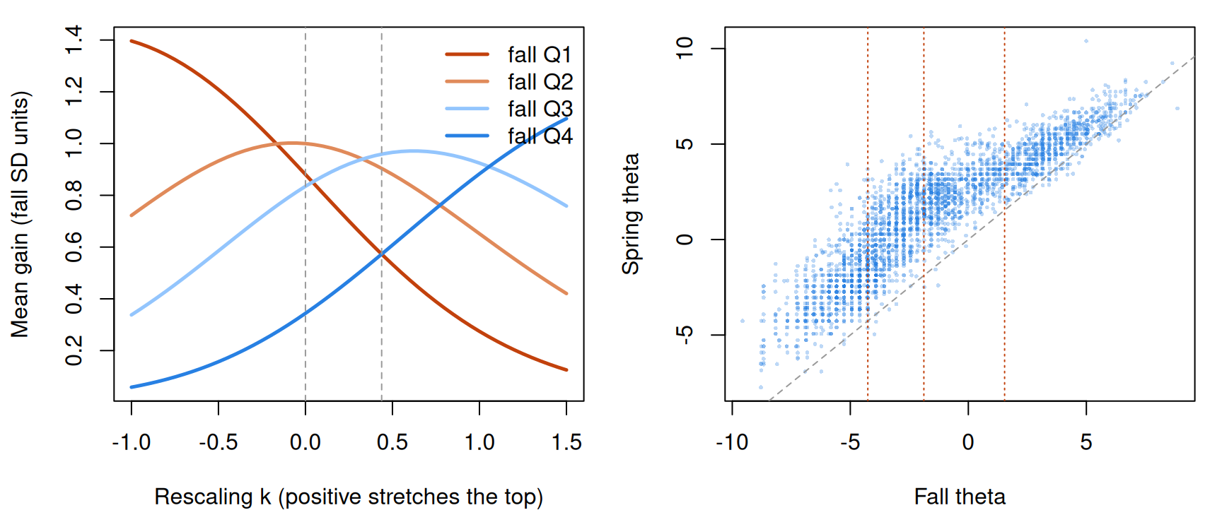

Code

par(op)

At \(k = 0.44\) the top quarter’s gain (0.57 fall SDs) catches the bottom quarter’s; at \(k = 1\) it is more than three times as large. The scatterplot shows why: the bottom quarter lives on a stretch of the scale the top quarter never visits.

Part of the bottom quarter’s lead is regression to the mean: fall scores low partly by chance tend to rise.

If you’ve done What does a score mean?: a difference between two error-laden scores is less reliable than either. The first score’s error enters the difference with a minus sign, so grouping on the first score builds error into the gains; grouping on a third measurement doesn’t.

Code

# Grouping on the fall score builds in regression to the mean: a fall score that
# is low partly by bad luck tends to be followed by a higher one. Group instead on
# the winter score, which shares no measurement error with fall or spring.
w2 <- kids[!is.na(kids$t2), ]
w2$q2 <- cut(w2$t2, quantile(w2$t2, 0:4 / 4), include.lowest = TRUE, labels = paste0("Q", 1:4))
round(rbind(fall_quartiles = tapply(w2$gain, w2$q, mean),
            winter_quartiles = tapply(w2$gain, w2$q2, mean)), 2)

                   Q1   Q2   Q3   Q4
fall_quartiles   3.21 3.64 3.02 1.26
winter_quartiles 2.76 3.49 3.22 1.64

Code

nrow(w2)

[1] 2940

Grouped on the winter score, the bottom quarter’s gain falls from 3.2 to 2.8 and the top’s rises from 1.3 to 1.6: same order, narrower gap.

Does the Rasch model give \(\theta\) a unit we can trust here?

Recall from The Rasch model: outfit well below 1 means an item is more predictable than the Rasch model expects (overfit, typically an item that discriminates better than average); well above 1 means noisier (underfit).

Code

# Does the Rasch model describe these items well enough to lend theta its unit?
# First, a 2PL, which lets every item have its own slope.
m2 <- mirt(X, 1, itemtype = "2PL", verbose = FALSE, technical = list(NCYCLES = 3000))
a <- coef(m2, simplify = TRUE)$items[, "a1"]
round(quantile(a, c(0.1, 0.5, 0.9)), 2)   # slopes, with the SD of theta fixed at 1

 10%  50%  90% 
2.41 4.16 7.09

Code

round(c(AIC_rasch = extract.mirt(m1, "AIC"), AIC_2pl = extract.mirt(m2, "AIC")))

AIC_rasch   AIC_2pl 
   226621    211105

Code

# Second, outfit and infit (the rasch lesson), using the WLE thetas.
fit_real <- itemfit(m1, fit_stats = "infit", Theta = matrix(recs$theta))
fit_summary <- function(f) round(c(median_outfit = median(f$outfit),
  overfit = sum(f$outfit < 0.7), underfit = sum(f$outfit > 1.3), items = nrow(f)), 2)
fit_summary(fit_real)

median_outfit       overfit      underfit         items 
         0.51        113.00          2.00        140.00

The 2PL’s AIC is lower by about 15,500, the slopes run from 2.4 to 7.1 (10th to 90th percentile), and 113 of the 140 items overfit. But the ceiling rule and credited early items might make responses more predictable whatever the items are. The known answer: a copy of the table simulated from the Rasch model with the fitted difficulties, each record’s \(\theta\), and the same forms, starting points and ceiling rule.

Code

# The known answer. Simulate a copy of the table from the Rasch model itself, with
# the fitted difficulties and each record's theta, and give it the same design:
# the same form, the same starting position, and the ceiling rule (stop at the end
# of the eight-item page on which a child first misses six in a row). Then run the
# same checks. Whatever misfit the copy shows comes from the design, not the items.
fm <- substr(colnames(X), 1, 1); ps <- as.integer(substr(colnames(X), 2, 3))
rec_form <- substr(df$it, 1, 1)[match(rownames(X), df$rec)]
rec_start <- first[rownames(X)]
S <- matrix(NA_integer_, nrow(X), ncol(X), dimnames = dimnames(X))
for (i in seq_len(nrow(X))) {
  cols <- which(fm == rec_form[i] & ps >= rec_start[i])
  cols <- cols[order(ps[cols])]
  x <- rbinom(length(cols), 1, plogis(recs$theta[i] - b[cols]))
  run <- cumsum(x == 0) - cummax((x == 1) * cumsum(x == 0))   # current run of misses
  hit <- which(run >= 6)[1]
  stop <- if (is.na(hit)) length(cols) else
    max(which(ps[cols] <= ceiling(ps[cols[hit]] / 8) * 8))
  S[i, cols[seq_len(stop)]] <- x[seq_len(stop)]
}
S <- as.data.frame(S)
c(items_per_record_real = mean(rowSums(!is.na(X))), items_per_record_copy = mean(rowSums(!is.na(S))))

items_per_record_real items_per_record_copy 
             43.15195              44.55271

Code

s1 <- mirt(S, 1, itemtype = "Rasch", verbose = FALSE)
s2 <- mirt(S, 1, itemtype = "2PL", verbose = FALSE, technical = list(NCYCLES = 3000))
theta_copy <- fscores(s1, method = "WLE", verbose = FALSE)[, 1]
fit_copy <- itemfit(s1, fit_stats = "infit", Theta = matrix(theta_copy))
lr <- function(r, t) 2 * (extract.mirt(t, "logLik") - extract.mirt(r, "logLik"))
rbind(real = c(AIC_rasch = extract.mirt(m1, "AIC"), AIC_2pl = extract.mirt(m2, "AIC"),
               LR = lr(m1, m2), fit_summary(fit_real)),
      copy = c(AIC_rasch = extract.mirt(s1, "AIC"), AIC_2pl = extract.mirt(s2, "AIC"),
               LR = lr(s1, s2), fit_summary(fit_copy)))

     AIC_rasch  AIC_2pl        LR median_outfit overfit underfit items
real  226620.5 211105.4 15793.099          0.51     113        2   140
copy  271316.2 268866.1  2728.083          0.66      78        0   140

The design matters: in the copy, where the Rasch model is true, 78 items overfit and the 2PL still improves the likelihood (a likelihood-ratio statistic of 2,728). The real table goes much further (15,793, and 113 overfitting items).

Fit statistics ask whether the Rasch curves match the data; the cancellation conditions ask whether any additive structure could. The ConjointChecks package tests them (Domingue, 2014); how much the resulting statistic can tell you at a given sample size, and how to calibrate it by bootstrap, is studied by Student and Read (2025). The package needs complete data, so we take a block that every record in it read: form A’s positions 2 to 40, for records that reached position 40. It runs when the page is built, not in the browser.

Code

# The cancellation conditions, tested with the ConjointChecks package (Domingue,
# 2014; install.packages("ConjointChecks")). It needs complete data, so we take a
# block that every record in it read: form A, positions 2 to 40, for the records
# whose run reached position 40, keeping items that between 2% and 98% of them
# read correctly. Rows are sum-score groups (at least 30 records each), columns
# the items. For each adjacent 3 x 3 submatrix the package draws proportions under
# the order restrictions (a Bayesian model, as in Karabatsos, 2001) and flags
# cells whose observed proportion falls outside the 95% credible interval. The
# summary is the average share of flagged cells.
library(ConjointChecks)
set.seed(2014)
blk <- which(fm == "A" & ps >= 2 & ps <= 40)
keep_rec <- rowSums(!is.na(X[, blk])) == length(blk)
B <- as.matrix(X[keep_rec, blk])
pc <- colMeans(B)
B <- B[, pc > 0.02 & pc < 0.98]
dim(B)   # records, items

[1] 3538   23

Code

# The known answer again: the same records and items simulated from the Rasch model.
Bc <- matrix(rbinom(length(B), 1, plogis(outer(recs$theta[keep_rec], b[colnames(B)], "-"))),
             nrow(B), dimnames = dimnames(B))
share_flagged <- function(R, single) {
  p <- PrepareChecks(R, ss.lower = 30)
  ConjointChecks(p$N, p$n, n.3mat = "adjacent", single = single)@means$unweighted
}
round(rbind(real = c(double = share_flagged(B, FALSE), single_and_double = share_flagged(B, TRUE)),
            copy = c(double = share_flagged(Bc, FALSE), single_and_double = share_flagged(Bc, TRUE))), 2)

     double single_and_double
real   0.17              0.17
copy   0.11              0.10

In the real block 0.17 of the cells fall outside their 95% credible intervals, against 0.11 in a Rasch-generated copy of the block (the check has false alarms, so the copy is the baseline); adding single cancellation changes little (0.17 and 0.10). Fit and cancellation agree: these items discriminate unequally, as naming a letter and reading a rare word might, and depart from additivity by more than chance. (Good cancellation with poor fit would instead point to an additive scale with a link other than the logistic.) The Rasch model’s licence for the unit is weaker here than for a Rasch-generated copy.

Finally, a comparison that needs almost no unit. Four of the studies randomized classrooms or schools to business-as-usual instruction or to Individualized Student Instruction (ISI), in which software recommends how much of each kind of reading instruction each child gets (Connor, Morrison, Fishman, Schatschneider & Underwood, 2007). (The two studies that compared ISI with a vocabulary intervention are left out; see For instructors.) Randomization gives the two arms the same fall distribution in expectation, case 1 of the Go deeper callout.

Code

# Projects 1, 2, 5 and 6 randomized classrooms or schools to Individualized
# Student Instruction (ISI) or business-as-usual reading instruction (van Dijk et
# al., 2022). In the IRW table treat = 1 is ISI there; children in project 5's third
# condition are coded missing and left out. Effect of ISI on the fall-to-spring gain,
# in fall-SD units, within project, under each rescaling. Randomization was by
# classroom or school, so these naive standard errors are too small: the point is
# the sign, not the p-value.
tr <- kids
tr$treat <- tapply(df$treat, df$id, function(x) x[1])[as.character(tr$id)]
tr <- tr[tr$project %in% c(1, 2, 5, 6) & tr$treat %in% c(0, 1), ]
table(project = tr$project, treat = tr$treat)

       treat
project   0   1
      1 238 305
      2 186 211
      5 319 254
      6 116 181

Code

tz1 <- (tr$t1 - mean(kids$t1)) / sd1; tz3 <- (tr$t3 - mean(kids$t1)) / sd1
effect <- function(k) {
  g <- (f_k(tz3, k) - f_k(tz1, k)) / sd(f_k(z1, k))
  coef(summary(lm(g ~ tr$treat + factor(tr$project))))[2, 1:2]
}
round(t(sapply(c(-1, -0.5, 0, 0.5, 1, 1.5), function(k) c(k = k, effect(k)))), 3)

        k Estimate Std. Error
[1,] -1.0    0.064      0.029
[2,] -0.5    0.065      0.022
[3,]  0.0    0.059      0.019
[4,]  0.5    0.042      0.019
[5,]  1.0    0.019      0.020
[6,]  1.5   -0.004      0.020

ISI’s effect on the gain is 0.06 fall SDs on \(\theta\), between 0.04 and 0.07 for \(k\) from −1 to 0.5, 0.02 at \(k = 1\) and −0.004 at \(k = 1.5\) (a unit at +2 SDs worth about 400 at −2 SDs). The sign holds over a far wider range than the comparison of quarters did. (These standard errors ignore clustering; the sign is the point.)

What do these data support? That the ISI arms gained more, by an amount that depends somewhat on the scale; and that children who started lower gained more, as a hypothesis whose sign turns on the spacing of a scale the Rasch model describes only partly. The same line runs through any such analysis: what survives every rescaling needs no assumption about the unit, while a comparison of gains across distant parts of a scale rests on that assumption, and so on the evidence for it from fit and the cancellation checks. A scale earns its unit one fit at a time.

Problems

Cancellation, derived and broken. Show that the Rasch model’s probabilities satisfy double cancellation for every choice of three respondents and three items. Then construct a 2PL example (three respondents, three items) in which double cancellation fails.
Gains on a 2PL scale. Redo the gain comparison with \(\theta\) from the 2PL. Does the order of the quarters’ gains change? Where does the crossing \(k\) move from 0.44, and why?
Caught up? A district reports that its lowest readers “caught up” with average readers between grades 3 and 5 on a vertically scaled test. What would you need to know before believing it? Which parts of the claim could be checked without an equal unit?
Design a test of the unit. You are building a reading scale for grades 1 to 6. What data, which check, and what result would persuade you that it is equal-interval?
A metric-free comparison. For the ISI contrast, compute Ho’s \(V = \sqrt 2\, \Phi^{-1}(P)\) for spring \(\theta\), where \(P\) is the probability that a random treated child outscores a random control child (Ho, 2009). Compare it with the standardized mean difference, and show that \(V\) doesn’t move under rescaling.
Challenge: what would convince them? Michell (2000) argues that psychometrics treats its attributes as quantitative without testing it; Borsboom and Mellenbergh (2004) answer that fitting item response models tests it jointly with other assumptions. What evidence would satisfy each, and would any satisfy both? This is open.

Stuck, or curious about something this lesson doesn’t cover? Ask Claude about this lesson opens a new conversation that already knows what the lesson is about; add your question at the end. Claude shows a caution notice on any prompt that arrives through a link; that’s expected.

Going further

Luce, R. D., & Tukey, J. W. (1964). Simultaneous conjoint measurement: A new type of fundamental measurement. Journal of Mathematical Psychology, 1(1), 1–27. https://doi.org/10.1016/0022-2496(64)90015-x. Where a unit from order alone comes from.
Perline, R., Wright, B. D., & Wainer, H. (1979). The Rasch model as additive conjoint measurement. Applied Psychological Measurement, 3(2), 237–255. https://doi.org/10.1177/014662167900300213. The connection, with two worked data sets.
Karabatsos, G. (2001). The Rasch model, additive conjoint measurement, and new models of probabilistic measurement theory. Journal of Applied Measurement, 2(4), 389–423. https://pubmed.ncbi.nlm.nih.gov/12011506/. Testing the cancellation conditions when responses carry error.
Domingue, B. (2014). Evaluating the equal-interval hypothesis with test score scales. Psychometrika, 79(1), 1–19. https://doi.org/10.1007/s11336-013-9342-4. A Bayesian check of the conditions, evaluated by simulation and applied to a reading test.
Student, S. R., & Read, W. S. (2025). Applying Bayesian checks of cancellation axioms for interval scaling in limited samples. Behavior Research Methods, 57, 305. https://doi.org/10.3758/s13428-025-02844-7. How the Bayesian cancellation checks behave with 250 or 1,000 respondents, and bootstrap procedures for deciding whether the result supports an interval scale.
Kyngdon, A. (2008). The Rasch model from the perspective of the representational theory of measurement. Theory & Psychology, 18(1), 89–109. https://doi.org/10.1177/0959354307086924. A dissent: the Rasch model read against the representational theory of measurement.
Michell, J. (2000). Normal science, pathological science and psychometrics. Theory & Psychology, 10(5), 639–667. https://doi.org/10.1177/0959354300105004. The argument Borsboom and Mellenbergh answer.
Lord, F. M. (1975). The ‘ability’ scale in item characteristic curve theory. Psychometrika, 40(2), 205–217. https://doi.org/10.1007/bf02291567. The metric of \(\theta\) as a choice.
Briggs, D. C. (2013). Measuring growth with vertical scales. Journal of Educational Measurement, 50(2), 204–226. https://doi.org/10.1111/jedm.12011. What a vertical scale’s interval claim would need.
Briggs, D. C., & Domingue, B. W. (2013). The gains from vertical scaling. Journal of Educational and Behavioral Statistics, 38(6), 551–576. https://doi.org/10.3102/1076998613508317. When the choice of vertical scale changes conclusions about gains.
Briggs, D. C., & Weeks, J. P. (2009). The impact of vertical scaling decisions on growth interpretations. Educational Measurement: Issues and Practice, 28(4), 3–14. https://doi.org/10.1111/j.1745-3992.2009.00158.x. Eight vertical scales from one data set.
Yen, W. M. (1986). The choice of scale for educational measurement: An IRT perspective. Journal of Educational Measurement, 23(4), 299–325. https://doi.org/10.1111/j.1745-3984.1986.tb00252.x. Criteria for choosing a scale, and scale shrinkage.
Bond, T. N., & Lang, K. (2013). The evolution of the Black-White test score gap in grades K–3: The fragility of results. Review of Economics and Statistics, 95(5), 1468–1479. https://doi.org/10.1162/rest_a_00370. Gap trends under rescaling.
Bond, T. N., & Lang, K. (2018). The Black–White education scaled test-score gap in grades K-7. Journal of Human Resources, 53(4), 891–917. https://doi.org/10.3368/jhr.53.4.0916.8242r. A unit borrowed from eventual educational attainment.
Ho, A. D. (2009). A nonparametric framework for comparing trends and gaps across tests. Journal of Educational and Behavioral Statistics, 34(2), 201–228. https://doi.org/10.3102/1076998609332755. Gap statistics that no rescaling changes.
Reardon, S. F., & Ho, A. D. (2015). Practical issues in estimating achievement gaps from coarsened data. Journal of Educational and Behavioral Statistics, 40(2), 158–189. https://doi.org/10.3102/1076998615570944. Metric-free gaps when only proficiency categories are reported.
Ballou, D. (2009). Test scaling and value-added measurement. Education Finance and Policy, 4(4), 351–383. https://doi.org/10.1162/edfp.2009.4.4.351. What scaling does to value-added estimates.
Jacob, B., & Rothstein, J. (2016). The measurement of student ability in modern assessment systems. Journal of Economic Perspectives, 30(3), 85–108. https://doi.org/10.1257/jep.30.3.85. What test scales can and can’t support, for economists.

Data sources

Data from the Item Response Warehouse (each table name links to its IRW page); references from IRW biblio.

project_kids_wj_lwid_wave: Hart, S. A., Otaiba, S. A., Connor, C., & Norris, C. U. (2021). Project KIDS Item level Data. LDbase. https://doi.org/10.33009/ldbase.1620837890.bcf8. Licence: CC BY 4.0.

For instructors

Source: new for this course (#66); no EDUC 252 slides. Built from the measurement-theory literature (Luce & Tukey; Michell; Borsboom & Mellenbergh; Perline, Wright & Wainer) and the literature on gains, growth and gaps (Yen; Briggs & Weeks; Briggs; Briggs & Domingue; Bond & Lang; Ho). The Project KIDS analysis is new.
Timing: about 60 minutes for the core ideas and widgets; the real-data section works as a 30-minute lab, and its code takes about ten minutes to run.
Data notes: the WJ-III form (A or B) is in the item names from IRW version 435 (item_response_warehouse v61.0); earlier versions pooled the forms by position. All ten WJ wave tables are split by form (IRW 436, v62.0); the six _grade tables and wj_sa still pool forms A and B by position (form B is at most 7 children per subtest), so don’t treat those as single-form item banks. The treatment contrast uses only the four studies that compared ISI with business-as-usual instruction (projects 1, 2, 5 and 6). In the two that compared ISI with a vocabulary intervention (projects 7 and 8), the group coded treat = 1 has the size that the data paper (van Dijk et al., 2022) gives for the vocabulary arm, so which arm is which is unclear from the table.
Held back: DIF as a source of group gaps (items, not the scale, differ across groups) is in Differential item functioning; treatment effects on latent scales, and constructs that change, are in Measurement invariance under treatment and life events; reporting scales (nonlinear transformations of \(\theta\)) are in What does a score mean?. A formal Bayesian test of the cancellation conditions across the IRW, following Domingue (2014), is not attempted.
Solutions: held back in solutions/scale-properties.qmd (not published).