Parameter invariance
What this is for
An item’s difficulty is supposed to belong to the item, not to whoever happened to answer it. That is the promise behind calibrating items once and using them for years, and behind the specific objectivity of The Rasch model. Does it hold? It depends on how you check. On the Multiracial Reading the Mind in the Eyes Test, item estimates from random halves of the sample agree almost perfectly, and estimates from women and from men nearly as well. Split the same respondents into high and low scorers on the test itself, and the 2PL’s estimates collapse: slopes near zero, difficulties unrelated. The items haven’t changed. The split has. This lesson separates what the model promises from what estimates can deliver, and shows why one way of splitting a sample undoes the check it was meant to perform.
Goals
By the end of this lesson you should be able to:
- say what parameter invariance claims, and why it is a property of the model rather than of any set of estimates;
- explain why two groups’ estimates sit on different scales, and derive how 2PL slopes and difficulties change with a group’s mean and SD of ability;
- explain why a group drawn from a narrow range of ability gives imprecise item estimates;
- explain why selecting respondents on the sum score of the same items distorts 2PL estimates, and why the Rasch model fitted by conditional maximum likelihood is not affected;
- check invariance in real data with
mirt, and say what each way of splitting a sample assumes.
Core ideas
Invariance belongs to the model
What does it mean for an item’s parameters to be the same in two groups? Think of a regression line. If \(y\) depends linearly on \(x\) in a population, a sample drawn only from small values of \(x\) and a sample drawn only from large ones estimate the same line, though each sees only part of it. An item characteristic curve is a regression of the response on \(\theta\), so the same holds: if the 2PL is true in a population, the same \(a\) and \(b\) govern responses in every subgroup of it, whatever its range of ability (Lord, 1980; Rupp & Zumbo, 2006).
Baker (2001, ch. 3, pp. 51–55) illustrates this with two groups of respondents, one with abilities from −3 to −1 and one from +1 to +3. Fitting the item’s curve to each group separately gives \(b = -0.39\) and \(a = 1.27\) both times: one group sees the lower tail, the other the upper tail, and both tails belong to one curve. The widget repeats the exercise. As in Baker’s illustration, the abilities are known, so each fit is a logistic regression on \(\theta\).
Try it: two groups, one curve
With sampling error off, both groups recover the true curve exactly, wherever you put them: that is Baker’s figure. Turn sampling error on and the estimates wobble, most for a group far from the item. At the defaults, group 2 sits where nearly everyone answers correctly, and its proportions say little about the curve’s shape. Add respondents and both fits close in on the dashed line. Invariance is a statement about the curve; estimates only approach it.
Compare the classical difficulty, the proportion correct. At the defaults it is about 0.15 in group 1 and above 0.9 in group 2 (read the points). Baker makes the same contrast: the proportion correct describes an item in a group, while \(b\) describes the item.
Estimates live on local scales
Baker’s groups share a scale because their abilities are known. In practice they aren’t, and each group’s fit sets the origin and unit by that group. Suppose group \(g\)’s abilities have mean \(\mu_g\) and SD \(\sigma_g\) on the population’s scale. The fit reports \(\theta^* = (\theta - \mu_g)/\sigma_g\), and to keep every \(a(\theta - b)\) unchanged it must report \[a^* = a\,\sigma_g, \qquad b^* = \frac{b - \mu_g}{\sigma_g}.\] A stronger group makes every item look easier by the same amount, and a more homogeneous group makes every slope look flatter. Under the Rasch model the slopes are fixed at 1, so only the shift remains. Nothing about the items has changed; the numbers are on local scales. Putting them on one scale is linking (Stocking & Lord, 1983; Kolen & Brennan, 2014).
Try it: two local scales
Before linking, the fifteen items lie on a straight line, just not the identity line: its intercept comes from the difference in means and its slope from the ratio of SDs. With B’s mean at 0 and SD at 1 the line is the identity. Link, and the points fall on it whatever the sliders say. A straight line in this plot is what invariance predicts. What it doesn’t predict is an item off the line.
Narrow groups give imprecise estimates
Baker’s groups were two logits wide. What if a group covers only a sliver of the scale? The slope is how fast the curve rises, and a group that spans a narrow range sees little rise to measure.
Try it: how wide a range?
At a width of 4 the estimates cluster around 1.27, with an SD of 0.15. Narrow the range to 1 and the SD triples; at 0.5 some samples give a slope below zero. Move the centre away from \(b = -0.39\) and the spread grows again, since a group far from the item sees only a flat stretch of curve. The item is the same in every setting; what shrinks is the information about it. A restricted group mostly costs precision.
Splitting on the sum score selects on the outcome
A narrow range of \(\theta\) costs precision. Selecting on the responses does something else. Suppose we split respondents into high and low scorers on the test we are calibrating. Within the high half the sum score can’t be low, so a respondent who missed one item must have made it up on others: among respondents with similar sum scores, answering one item correctly makes answering another less likely. Selection has introduced a dependence between items that has nothing to do with \(\theta\), so local independence no longer holds within the group. The sum score is a common effect of every item, and selecting on a common effect induces dependence between its causes, a problem known well beyond psychometrics (Elwert & Winship, 2014). A 2PL fit reads the items’ correlations as evidence of a common \(\theta\), and in a selected half those correlations are close to zero.
Try it: what selection does to the correlations
Splitting on true ability lowers the correlations, because each half has a narrower range of \(\theta\) (the previous section). Splitting on the sum score lowers them further, to about zero at the defaults. With four or five items it pushes them well below zero, since a fixed sum spread over a few items forces a trade-off between them. Raise the slope and every correlation rises, but the sum-score halves stay below the ability halves at every setting.
What about the Rasch model? There the sum score is sufficient, and conditional maximum likelihood estimates the difficulties from the responses given the sum score. Selecting respondents by that sum score leaves the conditional likelihood unchanged.
So the split that distorts a 2PL calibration is the one Andersen’s test is built on. The difference lies in what each fit conditions on. The 2PL’s marginal likelihood assumes the responses are independent given \(\theta\), and selection on the sum score undoes that. The Rasch conditional likelihood takes the sum score as given, so the selection has nothing left to undo.
When invariance fails for real
Estimation error, local scales and selection all make estimates differ when the items don’t. What is left after linking, in groups formed without selecting on the responses, is a difference in the items themselves. An item that is relatively harder for one group than another at the same \(\theta\) shows differential item functioning (Holland & Wainer, 1993), the subject of Differential item functioning. One limit is worth stating now. A shift common to every item can’t be told apart from a difference between the groups’ abilities, so invariance is checked item against item, never for the test as a whole.
Simulate
The code below simulates one population answering 20 items from a 2PL, then splits the respondents three ways: at random, on their true ability, and on their sum score. It fits the 2PL separately in each half and compares the estimates with the true parameters re-expressed on that half’s scale (\(a\sigma_g\) and \((b - \mu_g)/\sigma_g\), from the Go deeper callout). It runs in your browser; the first run takes a minute or more: 20–30 seconds while R and mirt load, then six fits.
With the seed as written, the random halves recover the slopes well (correlations of 0.94 and 0.91 with the truth). Halves split on true ability recover them less precisely (0.46 and 0.63) but at about the right level: median slopes of 0.65 and 0.56, against 0.56 and 0.58 on each half’s own scale. Halves split on the sum score get them too small: medians of 0.38 and 0.32, against 0.64 and 0.67. The last lines show why. The mean correlation between items is 0.149 in everyone, 0.052 in the upper half by ability and 0.019 in the upper half by sum score.
Try ni <- 5, and the sum-score halves get worse, as the widget suggested. Try np <- 10000 in your own R session: the ability halves close in on the truth, while the sum-score halves stay too flat, because more data doesn’t undo selection.
Download this code to run it in your own R session.
With real data
Our main example is wilmer-mrmet-normative-data-set-2022, the normative sample for the Multiracial Reading the Mind in the Eyes Test (MRMET; Kim et al., 2024). Like the RMET of From the 1PL to the 4PL, each item shows the eye region of a face and offers four words for the mental state it shows; the MRMET uses racially inclusive faces and answer choices that aren’t gendered. Its job here is to be a large sample with background variables, which we can split several ways to see which splits the item estimates survive. A response is 1 when the respondent chose the correct word. Download the code to run every chunk yourself.
Code
library(mirt)
# Each IRW table has a landing page (itemresponsewarehouse.org/tables/<name>/)
# with a CSV download. This link is pinned to one version of the data.
mrmet_url <- "https://redivis.com/api/v1/tables/datapages.item_response_warehouse_2:v24_0.wilmer-mrmet-normative-data-set-2022/rows?format=csv"
df <- read.csv(mrmet_url)
# resp is 1 when the respondent chose the correct word; resp_raw is the word chosen
# ("none" when no word was chosen, scored 0). The table is marked longitudinal because
# respondents took the test on different dates, but each took it once:
c(respondents = length(unique(df$id)), items = length(unique(df$item)),
  responses_per_respondent = unique(as.vector(table(df$id))),
  dates_per_respondent = max(tapply(df$date, df$id, function(x) length(unique(x)))))
respondents items responses_per_respondent
9295 37 37
dates_per_respondent
1 Code
long2wide <- function(df) {
  wide <- tapply(df$resp, list(df$id, df$item), function(x) x[1])
  as.data.frame(wide[, order(as.numeric(gsub("\\D", "", colnames(wide))))])
}
resp <- long2wide(df)
person <- df[!duplicated(df$id), c("id", "cov_gender", "cov_age", "cov_country")]
person <- person[match(rownames(resp), person$id), ]
r <- rowSums(resp)
round(range(colMeans(resp)), 2)          # proportion correct: easiest and hardest items
[1] 0.30 0.92Code
table(person$cov_gender)
     female genderqueer        male
       5505         419        3371
Code
# How strongly do the items go together? The mean correlation between pairs of items:
mean_r <- function(d) { R <- cor(d); mean(R[upper.tri(R)]) }
round(mean_r(resp), 3)
[1] 0.065All 9,295 respondents answered all 37 items. The IRW marks the table as longitudinal because respondents were tested on different dates, but each has one date. The items run from 30% to 92% correct, and they correlate weakly with one another: 0.065 on average, close to what the selection widget’s 20 items with slopes of 0.6 produce and less than half the simulation’s 0.149. Weak correlations leave a restricted sample less to work with.
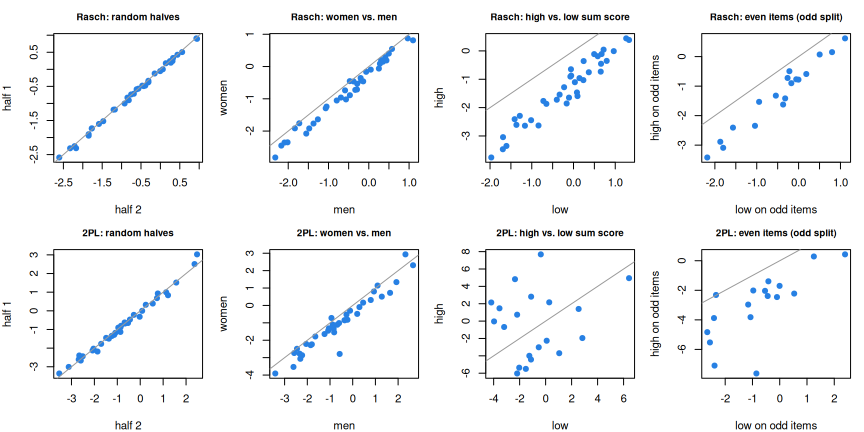
We fit the Rasch model and the 2PL in each half of four splits: random halves; women and men (the 419 respondents who reported genderqueer are left out of this split only, a group too small for its own 2PL calibration); high and low scorers on these 37 items; and, for the 18 even-numbered items, high and low scorers on the 19 odd-numbered ones.
Code
# Fit the Rasch model and the 2PL separately in two groups, and compare each item's
# estimates across the groups. IRTpars = TRUE converts mirt's intercept d to our
# difficulty, b = -d/a (for the Rasch model, b = -d).
fit_pars <- function(d, type) {
  coef(mirt(d, 1, itemtype = type, verbose = FALSE), simplify = TRUE, IRTpars = TRUE)$items[, c("a", "b")]
}
compare <- function(d, g, split, groups) {
  r1 <- fit_pars(d[g, ], "Rasch"); r2 <- fit_pars(d[!g, ], "Rasch")
  t1 <- fit_pars(d[g, ], "2PL");   t2 <- fit_pars(d[!g, ], "2PL")
  list(split = split, groups = groups, n = c(sum(g), sum(!g)), rasch = list(r1, r2), twopl = list(t1, t2),
       summary = data.frame(split = split, n1 = sum(g), n2 = sum(!g),
                            rasch_b_r = cor(r1[, "b"], r2[, "b"]),
                            rasch_shift = mean(r1[, "b"] - r2[, "b"]),
                            twopl_b_r = cor(t1[, "b"], t2[, "b"]),
                            twopl_a_r = cor(t1[, "a"], t2[, "a"]),
                            median_a_1 = median(t1[, "a"]), median_a_2 = median(t2[, "a"]),
                            mean_r_1 = mean_r(d[g, ]), mean_r_2 = mean_r(d[!g, ])))
}
set.seed(40)
random <- compare(resp, sample(c(TRUE, FALSE), nrow(resp), replace = TRUE), "random halves", c("half 1", "half 2"))
mf <- person$cov_gender %in% c("female", "male")
gender <- compare(resp[mf, ], person$cov_gender[mf] == "female", "women vs. men", c("women", "men"))
score  <- compare(resp, r > median(r), "high vs. low sum score", c("high", "low"))
odd <- seq(1, ncol(resp), by = 2); even <- seq(2, ncol(resp), by = 2)
r_odd <- rowSums(resp[, odd])
oddsplit <- compare(resp[, even], r_odd > median(r_odd), "even items, split on odd-item score",
                    c("high on odd items", "low on odd items"))
comps <- list(random, gender, score, oddsplit)
res <- do.call(rbind, lapply(comps, `[[`, "summary"))
print(format(res, digits = 2), row.names = FALSE)
split n1 n2 rasch_b_r rasch_shift twopl_b_r
random halves 4657 4638 1.00 -0.029 0.994
women vs. men 5505 3371 0.99 -0.242 0.963
high vs. low sum score 4168 5127 0.96 -1.178 -0.048
even items, split on odd-item score 3828 5467 0.98 -0.816 0.772
twopl_a_r median_a_1 median_a_2 mean_r_1 mean_r_2
0.97 0.609 0.60 0.0659 0.065
0.92 0.605 0.64 0.0604 0.068
0.63 -0.037 0.19 -0.0026 0.018
0.76 0.518 0.57 0.0289 0.053Code
# Each item's difficulty in one group against the other. Grey line: identity.
# Top row, the Rasch model; bottom row, the 2PL.
op <- par(mfrow = c(2, 4), mar = c(4, 4, 2.5, 1), cex = 0.7)
for (model in c("rasch", "twopl")) for (cc in comps) {
  x <- cc[[model]][[2]][, "b"]; y <- cc[[model]][[1]][, "b"]
  keep <- abs(x) < 8 & abs(y) < 8   # a slope near 0 sends b = -d/a off the page
  plot(x[keep], y[keep], pch = 19, col = "#2780e3", xlab = cc$groups[2], ylab = cc$groups[1],
       main = paste(if (model == "rasch") "Rasch:" else "2PL:", sub(", split on odd-item score", " (odd split)", cc$split)),
       cex.main = 0.85)
  abline(0, 1, col = "grey60")
}
Code
par(op)Read the table a row at a time.
- Random halves. Rasch difficulties correlate 1.00, 2PL difficulties 0.99 and 2PL slopes 0.97. This is the baseline: two samples from one population, differing only by estimation error.
- Women and men. Rasch difficulties correlate 0.99, with a shift of −0.24: on the women’s scale every item is about a quarter of a logit easier, which the model reads as women scoring higher on average, not as items that differ. The 2PL slopes agree less well (0.92), but slopes are the noisier parameter even between random halves (0.97).
- High and low scorers. The Rasch difficulties still correlate 0.96, shifted by 1.18 logits, the difference between the groups’ means. The 2PL collapses: its difficulties correlate −0.05, and the median slope is −0.04 in the high half and 0.19 in the low half. The mean correlation between items is −0.003 in the high half, as the selection widget predicted.
- Even items, split on the odd items. Selecting on other items avoids the common-effect problem, but the halves are narrower in ability, since the odd-item score tracks \(\theta\). The 2PL difficulties correlate 0.77 and the slopes 0.76, better than the sum-score split and worse than random halves: the cost of a restricted range.
Code
# In the high and low halves by sum score, the 2PL slopes:
round(rbind(high = quantile(score$twopl[[1]][, "a"], c(0, .25, .5, .75, 1)),
            low  = quantile(score$twopl[[2]][, "a"], c(0, .25, .5, .75, 1))), 2)
0% 25% 50% 75% 100%
high -0.68 -0.15 -0.04 0.41 0.75
low -0.43 0.01 0.19 0.43 1.18Code
# The same items in everyone, for comparison:
full_2pl <- fit_pars(resp, "2PL")
round(quantile(full_2pl[, "a"], c(0, .25, .5, .75, 1)), 2)
0% 25% 50% 75% 100%
0.21 0.42 0.60 0.92 1.19 Among high scorers the 2PL slopes run from −0.68 to 0.75; in the full sample the same items run from 0.21 to 1.19, median 0.60. A negative slope says that stronger respondents are less likely to answer correctly, and selection produced it here from items that all rise with ability in the full sample. With slopes near zero, \(b = -d/a\) divides by almost nothing, which is why some difficulties fall off the plot, as Y15’s did in From the 1PL to the 4PL.
What does the Rasch model’s 0.96 on that split mean? Under conditional ML the split is Andersen’s test, and legitimate:
Code
# Conditional maximum likelihood (psychotools::raschmodel) conditions on the sum
# score, so selecting respondents by that same sum score leaves its likelihood intact.
# Splitting there is Andersen's (1973) test of the Rasch model.
library(psychotools)
cml <- function(d) { m <- raschmodel(d); list(b = itempar(m), ll = logLik(m)) }
hi <- cml(resp[r > median(r), ]); lo <- cml(resp[r <= median(r), ]); all <- cml(resp)
round(cor(hi$b, lo$b), 3)
[1] 0.963Code
# Andersen's likelihood-ratio statistic, on (items - 1) degrees of freedom:
c(LR = round(2 * (as.numeric(hi$ll) + as.numeric(lo$ll) - as.numeric(all$ll))), df = ncol(resp) - 1)
LR df
1588 36 Code
# Which items move between the halves? Compare with each item's 2PL slope in everyone.
moved <- (hi$b - mean(hi$b)) - (lo$b - mean(lo$b))
round(cor(moved, full_2pl[, "a"]), 2)
[1] -0.98The conditional ML difficulties from the two halves correlate 0.963, and the likelihood-ratio statistic is 1,588 on 36 degrees of freedom, far beyond what the Rasch model allows. Which items move? The shift in each item’s difficulty between the halves correlates −0.98 with its 2PL slope in the full sample. Items that discriminate well look relatively easier to high scorers and harder to low scorers, which is what crossing curves do. Specific objectivity fails here in the way From the 1PL to the 4PL anticipated: the MRMET’s items differ in slope.
So which split checks invariance? The assumptions first. A 2PL fit in each group assumes the responses are independent given \(\theta\) within the group; the Rasch model fitted by conditional ML needs that only given the sum score. A split on the sum score of the calibrated items keeps the second and breaks the first, which is why the MRMET’s 2PL slopes collapsed on that split and its Rasch difficulties did not. Random halves give a baseline for estimation error; a background variable (gender, age, country) or a score on other items tests invariance without selecting on the calibrated responses. If the model is Rasch and the estimator is conditional ML, the sum-score split is Andersen’s test.
Problems
- Asymptotes and the Rasch model. Using the Go deeper callout, show that a 3PL’s lower asymptote \(c\) is the same on every group’s scale. Then show that under the Rasch model, where
mirtfixes the slopes at 1 and estimates the SD of \(\theta\), two groups’ difficulties differ only by a shift. Where does the group’s SD go? - Linking women and men. Link the men’s MRMET 2PL difficulties to the women’s scale by mean–sigma. How close do the items get? Which item is furthest off after linking, and what is its slope?
- Age. Split the MRMET respondents into those under 25 and those over 40, and repeat the comparison. After removing the Rasch shift, which items differ most? Are the difficulties invariant, and how would you tell a real difference from estimation error?
- A colleague’s split. A colleague checks a new test’s calibration by fitting the 2PL separately to the top and bottom thirds of scorers, finds slopes near zero in both, and concludes that the items don’t measure anything. What would you tell them, and what would you run instead?
- Calibrating for a new population. A test calibrated on adults will be used with 12- to 15-year-olds. You can collect data from 1,500 respondents. Whom would you sample, and why? What would you compare before trusting the adult parameters?
- Challenge: fewer parameters, more invariance? On every split, the Rasch difficulties agree better than the 2PL’s. Is that a property of the MRMET’s items, or of estimating one parameter per item instead of two? Wright (1997) makes the case for measurement whose item comparisons don’t depend on the sample. Design a simulation that could tell the two apart. This one is open: I don’t know of a general answer.
Going further
- Baker, F. B. (2001). The basics of item response theory (2nd ed.). ERIC Clearinghouse on Assessment and Evaluation. https://eric.ed.gov/?id=ED458219. Chapter 3 has the two-group illustration and a warning about what estimates can show; free to read. The third edition, with R code, is Baker, F. B., & Kim, S.-H. (2017), The basics of item response theory using R, Springer, https://doi.org/10.1007/978-3-319-54205-8.
- Rupp, A. A., & Zumbo, B. D. (2006). Understanding parameter invariance in unidimensional IRT models. Educational and Psychological Measurement, 66(1), 63–84. https://doi.org/10.1177/0013164404273942. Invariance stated exactly, as equality up to the model’s linear transformations, and what item parameter drift does to response probabilities.
- Lord, F. M. (1980). Applications of item response theory to practical testing problems. Erlbaum. https://doi.org/10.4324/9780203056615. Chapters on equating, tailored testing and item bias, each of which relies on item parameters that carry over from one group to another.
- Andersen, E. B. (1973). A goodness of fit test for the Rasch model. Psychometrika, 38(1), 123–140. https://doi.org/10.1007/BF02291180. Comparing difficulties across score groups, as a likelihood-ratio test.
- Stocking, M. L., & Lord, F. M. (1983). Developing a common metric in item response theory. Applied Psychological Measurement, 7(2), 201–210. https://doi.org/10.1177/014662168300700208. Putting two calibrations on one scale.
- Kolen, M. J., & Brennan, R. L. (2014). Test equating, scaling, and linking (3rd ed.). Springer. https://doi.org/10.1007/978-1-4939-0317-7. Linking methods in full.
- Holland, P. W., & Wainer, H. (Eds.). (1993). Differential item functioning. Erlbaum; Routledge reprint. https://doi.org/10.4324/9780203357811. What is left when invariance fails for real.
- Elwert, F., & Winship, C. (2014). Endogenous selection bias: The problem of conditioning on a collider variable. Annual Review of Sociology, 40, 31–53. https://doi.org/10.1146/annurev-soc-071913-043455. The general form of the sum-score split’s problem.
- Wright, B. D. (1997). A history of social science measurement. Educational Measurement: Issues and Practice, 16(4), 33–45. https://doi.org/10.1111/j.1745-3992.1997.tb00606.x. The case for measurement whose item comparisons don’t depend on the sample.
- Chalmers, R. P. (2012). mirt: A multidimensional item response theory package for the R environment. Journal of Statistical Software, 48(6). https://doi.org/10.18637/jss.v048.i06. The package for the marginal ML fits.
- Zeileis, A., Strobl, C., Wickelmaier, F., Komboz, B., Kopf, J., Schneider, L., & Debelak, R. psychotools: Infrastructure for psychometric modeling. R package. https://CRAN.R-project.org/package=psychotools. The conditional ML fits.
- Kim, H. A., Kaduthodil, J., Strong, R. W., Germine, L. T., Cohan, S., & Wilmer, J. B. (2024). Multiracial Reading the Mind in the Eyes Test (MRMET): An inclusive version of an influential measure. Behavior Research Methods, 56(6), 5900–5917. https://doi.org/10.3758/s13428-023-02323-x. The source of the MRMET data.
Data sources
Data from the Item Response Warehouse (each table name links to its IRW page); references from IRW biblio.
wilmer-mrmet-normative-data-set-2022: Kim, H.A., Kaduthodil, J., Strong, R.W. et al. Multiracial Reading the Mind in the Eyes Test (MRMET): An inclusive version of an influential measure. Behav Res 56, 5900–5917 (2024). https://doi.org/10.3758/s13428-023-02323-x. Licence: CC BY 4.0.
For instructors
- Source: EDUC 252 class 4 (slides c4, 35–43, “Parameter invariance”, including the Baker illustration) and
c4/enem2.Rinben-domingue/252. - Timing: the core ideas and widgets take about 50 minutes; the MRMET analysis works as a 25-minute lab. Its sixteen fits take a minute or two in local R.
- Changed from 252 (Ben, 09-24): the slides use ENEM; this lesson uses the MRMET, which has a tokenless CSV and background variables to split on. Linking forms is left to Linking and equating. The sum-score split, and its contrast with Andersen’s test, is this lesson’s own finding in the data (C17).
- Held back: linking methods (Linking and equating); testing individual items across groups (Differential item functioning); invariance of person parameters across item sets (Linking and equating, Item banks and adaptive testing).
- Solutions: held back in
solutions/parameter-invariance.qmd(not published).