Guessing and priors
What this is for
On the Reading the Mind in the Eyes Test, where chance is one in four, the 3PL’s median lower asymptote was 0.01. Yet respondents do guess. What to do about it turns on what we assume about who guesses and how: estimate \(c\) for each item, fix it at the chance rate, leave it out, or give guessing to respondents. Each is an assumption, and held-out responses can compare them. This lesson does so on a two-button reading task and a vocabulary test.
Goals
By the end of this lesson you should be able to:
- say which respondents the data use to estimate a lower asymptote, and predict when its estimate will be imprecise;
- fit a Rasch model with the lower asymptote fixed at chance, and say what it assumes;
- use response times to find rapid responses, and explain why guessing can be a property of respondents rather than items;
- choose lognormal and beta priors for slopes and lower asymptotes, and say what they do to the estimates;
- judge a guessing correction or a prior by out-of-sample prediction.
Core ideas
What does the lower asymptote learn from?
Why so little? A response carries information about \(c\) only where the logistic part of the curve is near zero; a respondent well above an item answers it correctly whatever \(c\) is. So the precision of \(\hat c\) is set by how many respondents find the item too hard, not by how many there are.
Try it: where the lower asymptote is learned
One 3PL item (\(a = 1.2\), \(b = 0\)), answered by \(n\) respondents whose abilities are normal around a mean you choose, relative to the item. The curve is the standard error of the estimated \(c\), from the Fisher information for \((a, b, c)\) with the abilities known. With estimated abilities it would be larger.
The opening setting, 1.5, is an easy test like the RMET: almost nobody is near the floor, and with 1,000 respondents the standard error of \(\hat c\) is 0.27. At −1 the test is hard for its takers, like the two hardest ENEM forms in the IRW’s guessing vignette, where about two-fifths of the items are answered correctly less often than chance; a fifth of the respondents are near the floor and the standard error falls to 0.05. Back at 1.5, even 20,000 respondents leave it at 0.06.
Domingue et al. (2024, §3) asked the question by simulation. With data generated from a 3PL whose lower asymptotes ran up to 0.3, the average IMV of the 3PL over the 2PL on held-out responses never exceeded 0.001, while the 2PL gained 0.01 or more over the 1PL when slopes varied substantially. They relate this to difficulties in identifying the 3PL (Maris & Bechger, 2009; Haberman, 2005; von Davier, 2009). The widget suggests why: a curve that differs from a 2PL only where few respondents are changes few predictions. Where many respondents sit near chance, or calibration samples are large, the data have more to say about \(c\), and the same comparison can come out differently.
Fix guessing from the item’s structure
If we know where the floor should be, why not put it there? With \(k\) equally attractive options, random choice is right with probability \(1/k\), and the simplest model with guessing fixes every lower asymptote there: \[\Pr(x_{ij} = 1) = \frac{1}{k} + \Big(1 - \frac{1}{k}\Big)\frac{\exp(\theta_j - b_i)}{1 + \exp(\theta_j - b_i)}.\] It is the Rasch model with a fixed floor, the first of three ways to add guessing that San Martín, del Pino and De Boeck (2006) list (the others estimate one floor for all items, or one per item). Han (2012) reports that fixing \(c = 1/k\) gave more stable item estimates than a free 3PL without a loss of fit, on simulated and real multiple-choice data.
What does fixing the floor assume? That a respondent who doesn’t know the answer picks at random. That doesn’t hold if some wrong options attract more than others, if respondents can rule some out (San Martín et al. let the chance of a correct guess rise with ability), or if not knowing pushes respondents toward one answer.
Try it: what a correct answer is worth
The same item (\(b = 0\)) under the Rasch model and with its floor fixed at chance. Choose the chance rate (four options for a typical multiple-choice test, two for the lexical decision task below) and how far below the item a respondent sits.
With two options and a gap of 3, one correct answer favours the higher ability by a factor of 10.5 under the Rasch model and by 1.43 with the floor at 0.5. With a floor of 0.25 its worth falls less (a factor of 2.2). Wrong answers lose nothing: the floor multiplies their probability by the same \(1 - c\) at every ability (problem 1).
Guessing may belong to respondents
The 3PL and the fixed floor both give guessing to items. But a respondent who has stopped trying, or is racing a clock, may answer items they could solve, quickly and at chance. Response times can find them: Schnipke and Scrams (1997) modelled times as a mixture of rapid guesses and slower solution behaviour, Wise and Kong (2005) measured engagement by the share of responses too fast to reflect reading, and Wise (2017) reviews the methods.
If guessing belongs to respondents, an item’s lower asymptote spreads a few respondents’ behaviour over everyone. Response time and the speed-accuracy tradeoff models times and responses together.
Two models put guessing with respondents without response times. In the ability-based guessing model (1PL-AG) of San Martín, del Pino and De Boeck (2006), a respondent who doesn’t know the answer guesses right with a probability that rises with ability, as if stronger respondents rule out more options: \[\Pr(x_{ij} = 1) = P_{ij} + (1 - P_{ij})\,\frac{\exp(\alpha\theta_j + \gamma_i)}{1 + \exp(\alpha\theta_j + \gamma_i)}, \qquad P_{ij} = \frac{\exp(\theta_j - b_i)}{1 + \exp(\theta_j - b_i)}.\] In a two-class mixture, each respondent either follows the Rasch model, with probability \(\pi\), or answers every item correctly with the chance probability \(c\). For a respondent whose class we don’t know, and if the classes don’t differ in ability, the probability of a correct answer is \(\pi P_{ij} + (1 - \pi)c\).
Try it: four ways to add guessing
One item with difficulty \(b\). The widget sets \(\gamma_i\) so that a respondent at \(\theta = 0\) who doesn’t know the answer guesses right with probability \(c\), as under the fixed floor.
The curves part company at the two ends. At the bottom, the fixed floor lifts every respondent to \(c\), while the mixture lifts them only to \((1 - \pi)c\), 0.04 at the defaults, because only the guessing class guesses. At the top, the mixture never reaches 1: a guesser misses easy items too, so its ceiling is \(\pi + (1 - \pi)c\), 0.89 at the defaults. The 1PL-AG has no fixed floor at all: guessing fades for weak respondents and helps strong ones. Set \(\alpha\) to 0 and it becomes the fixed floor; set \(\pi\) to 1 and the mixture becomes the Rasch model.
Priors keep item estimates in bounds
Nothing in that argument needs \(\theta\) to be an ability. An item parameter can have a prior too, and its posterior is again likelihood times prior (Mislevy, 1986; Swaminathan & Gifford, 1986; Harwell & Baker, 1991). A slope is positive, so \(\log a\) gets a normal prior (a lognormal on \(a\)); a lower asymptote lies between 0 and 1, so it gets a beta prior; beta(\(\alpha\), \(\beta\)) has mean \(\alpha/(\alpha + \beta)\), mode \((\alpha - 1)/(\alpha + \beta - 2)\), and counts for roughly \(\alpha + \beta\) responses, so beta(2, 18) says “about 0.1, worth about 20 responses”. Since mirt finds the posterior mode, a lower asymptote the data say little about settles near the prior’s mode, 0.056 for beta(2, 18). Where data are thin, which for \(c\) is nearly always, the estimate sits near the prior; priors do the most when a sample is small for the number of item parameters, and where a prior sits is itself an assumption. A full Bayesian treatment is in Johnson and Sinharay (2017).
Try it: prior × likelihood = posterior for a slope
One item (\(b = 0\), no floor), answered by \(n\) respondents with known abilities, from a fixed sample of 2,000. Twenty respondents is a small pilot; 300 is the size of the vocabulary subsamples below. The prior on \(\log a\) is normal with mean 0 and the SD you choose.
With 20 respondents the maximum-likelihood slope is 3.17, more than twice the truth, and the posterior mode is 2.16, pulled back toward 1. With 300 they agree within a few hundredths. Tighten the prior’s SD to 0.25 and at 20 respondents the prior wins: the mode is 1.15, now below the truth. This is shrinkage again, now for items, and a tight prior in the wrong place pulls every estimate toward the wrong place.
Judge it by prediction
Fixing \(c\) and adding priors are both assumptions, which the model’s own fit statistics take for granted. The check that doesn’t is the one from Model fit and out-of-sample prediction: fit with and without the assumption, and compute the IMV on held-out responses.
Simulate
The code below simulates a five-option test from the 3PL (20 items, every \(c = 0.2\)) for 300 respondents, then fits the 2PL, the 3PL without priors, and the 3PL with a lognormal(0, 1) prior on the slopes and a beta(4, 16) prior on the lower asymptotes (mean 0.2, the chance rate; mode 0.17). The first run takes 20–30 seconds while R and mirt load, and the fits up to a minute more.
With the seed as written, the 3PL without priors has a slope as large as 6.8 (the true slopes are around 1), a slope error of 1.74 and a median \(c\) of 0.29. With the priors, the slope error is 0.31, the difficulty error falls from 1.04 to 0.51, and the median \(c\) is 0.17. All three give abilities that correlate 0.76 to 0.78 with the truth. With np <- 3000 (in your own R session) the 3PL’s slope error falls to 0.32 on its own and the priors still help (0.22). Try expbeta, 2, 18 (mean 0.1) to see what a prior in the wrong place costs.
Download this code to run it in your own R session.
With real data
A two-button reading task
Our main example is roar_lexical, from the lexical decision task of the Rapid Online Assessment of Reading (Yeatman et al., 2021): children and adolescents saw a string of letters and pressed one of two buttons to say whether it was a real word, under a time limit. Its job is to be a test whose chance rate is known exactly: 0.5. Every response has a time. Download the code to run every chunk yourself; it needs mirt (Chalmers, 2012).
Code
library(mirt)
# Each IRW table has a landing page (itemresponsewarehouse.org/tables/<name>/) with
# a CSV download. This link is pinned to one version of the data.
roar_url <- "https://redivis.com/api/v1/tables/datapages.item_response_warehouse:v60_0.roar_lexical/rows?format=csv"
roar <- read.csv(roar_url)
# One row per response. resp is 1 when the respondent classified the string
# correctly (real word or made-up word); rt is the response time in seconds;
# realpseudo says which kind of string it was. One response per respondent per
# item, and no waves.
c(responses = nrow(roar), respondents = length(unique(roar$id)),
  items = length(unique(roar$item)), missing = sum(is.na(roar$resp)))
responses respondents items missing
61500 123 500 0 Code
table(roar$realpseudo)
pseudo   real
 30750  30750
Code
round(c(accuracy = mean(roar$resp), tapply(roar$resp, roar$realpseudo, mean)), 2)accuracy pseudo real
0.80 0.77 0.82 Code
# IRW tables are long (one row per response); mirt wants wide (one row per respondent).
long2wide <- function(df) as.data.frame(tapply(df$resp, list(df$id, df$item), function(x) x[1]))
resp_roar <- long2wide(roar)
round(quantile(colMeans(resp_roar), c(0, 0.1, 0.5, 1)), 2)   # proportion correct by item
0% 10% 50% 100%
0.14 0.64 0.84 0.96 There are 123 respondents, each classifying the same 500 strings (half real words), with no missing responses and one wave. Overall accuracy is 0.80.
Code
# The Rasch model, and the Rasch model with every lower asymptote fixed at 0.5
# (two choices, so chance is one in two). guess = 0.5 fixes mirt's g, our c; it is
# not estimated, so both models have the same number of parameters.
set.seed(252)
rasch <- mirt(resp_roar, 1, itemtype = "Rasch", verbose = FALSE)
fixed <- mirt(resp_roar, 1, itemtype = "Rasch", guess = 0.5, verbose = FALSE)
b_rasch <- -coef(rasch, simplify = TRUE)$items[, "d"]   # mirt's d is an easiness: b = -d
b_fixed <- -coef(fixed, simplify = TRUE)$items[, "d"]
th_rasch <- fscores(rasch)[, 1]
th_fixed <- fscores(fixed)[, 1]
data.frame(parameters = c(extract.mirt(rasch, "nest"), extract.mirt(fixed, "nest")),
           logLik = round(c(extract.mirt(rasch, "logLik"), extract.mirt(fixed, "logLik"))),
           sd_ability = round(sqrt(c(coef(rasch)$GroupPars[2], coef(fixed)$GroupPars[2])), 2),
           sd_difficulty = round(c(sd(b_rasch), sd(b_fixed)), 2),
row.names = c("Rasch", "Rasch, c = 0.5"))| parameters | logLik | sd_ability | sd_difficulty | |
|---|---|---|---|---|
| Rasch | 501 | -25579 | 0.92 | 0.80 |
| Rasch, c = 0.5 | 501 | -25380 | 1.67 | 2.03 |
Code
round(c(cor_abilities = cor(th_rasch, th_fixed), cor_difficulties = cor(b_rasch, b_fixed)), 2) cor_abilities cor_difficulties
0.97 0.87 The two models rank respondents almost identically (the abilities correlate 0.97), and the fixed floor fits better, with a log likelihood of −25,380 against −25,579 for the same number of parameters. The scale spreads out: the SD of ability goes from 0.92 to 1.67, and of difficulty from 0.8 to 2.0.
Code
# Where do the two models disagree about an item? Difficulty against proportion
# correct: with c = 0.5, an item that 60% get right is only just above chance.
p_roar <- colMeans(resp_roar)
plot(p_roar, b_rasch, pch = 19, col = "#93c5fd", ylim = range(c(b_rasch, b_fixed)),
     xlab = "Proportion correct", ylab = "Difficulty b")
points(p_roar, b_fixed, pch = 19, col = "#2780e3")
legend("topright", c("Rasch", "Rasch, c = 0.5"), pch = 19, col = c("#93c5fd", "#2780e3"), bty = "n")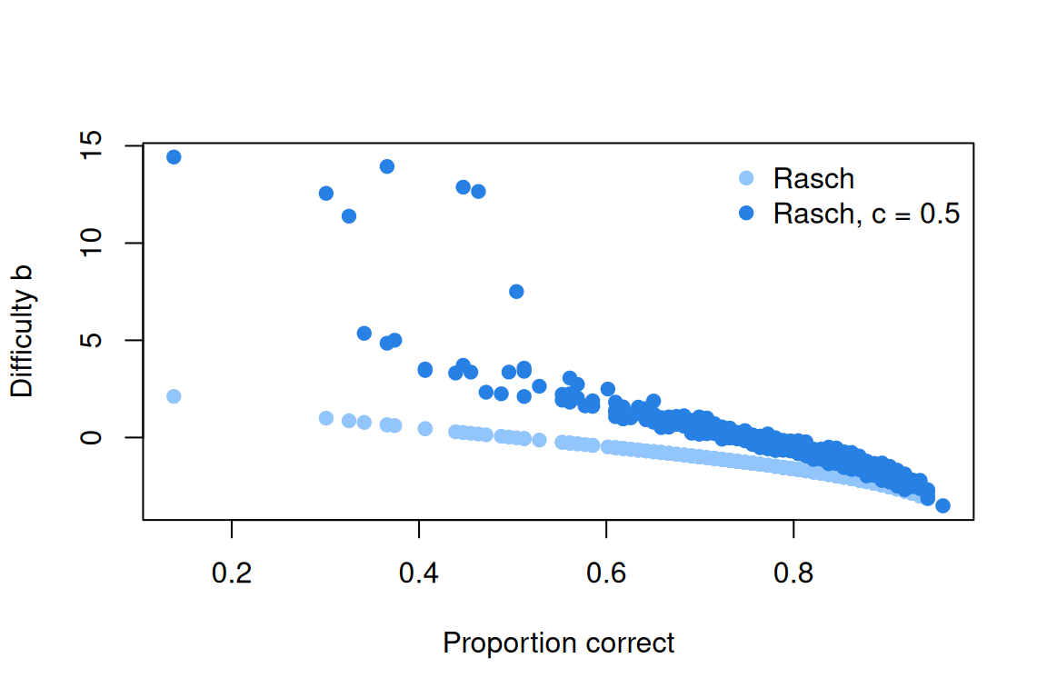
Code
# Items answered correctly by fewer than half the respondents: below chance. Are
# they real words or made-up ones?
kind <- tapply(roar$realpseudo, roar$item, function(x) x[1])[names(p_roar)]
table(kind[p_roar < 0.5])
pseudo   real
     6     11
Code
# The five hardest items under each model
hardest <- order(p_roar)[1:5]
data.frame(p = round(p_roar[hardest], 2), b_rasch = round(b_rasch[hardest], 2),
b_fixed = round(b_fixed[hardest], 2))| p | b_rasch | b_fixed | |
|---|---|---|---|
| napery | 0.14 | 2.11 | 14.42 |
| yammering | 0.30 | 0.99 | 12.56 |
| acquisitiveness | 0.33 | 0.86 | 11.38 |
| impoverish | 0.34 | 0.78 | 5.36 |
| hitter | 0.37 | 0.65 | 13.94 |
The hardest items show where the spread comes from. Seventeen strings, 11 real words and 6 made-up ones, are classified correctly by fewer than half the respondents, below what random pressing would give; the real word napery by 14%. A respondent who doesn’t know a word says it isn’t one, and a word-like made-up string gets called a word. A floor at 0.5 can’t describe an item below chance, so the fixed floor sends the five hardest to difficulties of 5.4 to 14.4: its assumption, that not knowing means choosing at random, doesn’t hold for these items.
Code
# Does fixing c help on responses the models never saw? Five-fold cross-validation
# over responses, scored by the IMV (as in the lesson "Model fit and out-of-sample
# prediction").
coin <- function(ll) {
  if (ll <= log(0.5)) return(0.5)
  uniroot(function(w) w * log(w) + (1 - w) * log(1 - w) - ll, c(0.5, 1 - 1e-12), tol = 1e-12)$root
}
mean_ll <- function(y, p) mean(y * log(p) + (1 - y) * log(1 - p))
imv <- function(y, p0, p1) {
  w0 <- coin(mean_ll(y, p0)); w1 <- coin(mean_ll(y, p1))
  (w1 - w0) / w0
}
# Predicted probabilities for cells (row, column) from a fitted model, in mirt's
# form g + (u - g) * logistic(a * theta + d), with EAP abilities.
predict_cells <- function(m, cells) {
  th <- fscores(m)[, 1]
  cf <- coef(m, simplify = TRUE)$items
  i <- cells[, 2]
  cf[i, "g"] + (cf[i, "u"] - cf[i, "g"]) * plogis(cf[i, "a1"] * th[cells[, 1]] + cf[i, "d"])
}
set.seed(1)
X <- as.matrix(resp_roar)
cells <- which(!is.na(X), arr.ind = TRUE)
fold <- sample(rep(1:5, length.out = nrow(cells)))
cv <- do.call(rbind, lapply(1:5, function(f) {
  test <- cells[fold == f, , drop = FALSE]
  train <- X; train[test] <- NA; train <- as.data.frame(train)
  data.frame(fold = f, row = test[, 1], col = test[, 2], y = X[test],
             rasch = predict_cells(mirt(train, 1, itemtype = "Rasch", verbose = FALSE), test),
             fixed = predict_cells(mirt(train, 1, itemtype = "Rasch", guess = 0.5, verbose = FALSE), test))
}))
imv_folds <- sapply(split(cv, cv$fold), function(d) imv(d$y, d$rasch, d$fixed))
round(c(imv_folds, mean = mean(imv_folds)), 4)
1 2 3 4 5 mean
0.0027 0.0024 0.0023 0.0028 0.0011 0.0023 Code
# Where does the gain come from? The same IMV among held-out responses from the
# quarter of respondents with the lowest accuracy, and from everyone else.
acc <- rowMeans(X)
low <- acc[cv$row] <= quantile(acc, 0.25)
round(c(lowest_quarter = imv(cv$y[low], cv$rasch[low], cv$fixed[low]),
        other_three_quarters = imv(cv$y[!low], cv$rasch[!low], cv$fixed[!low])), 4)
lowest_quarter other_three_quarters
0.0574 -0.0017 Out of sample, the fixed floor beats the Rasch model in all five folds, by an IMV of 0.0023 on average: a fifth of the 0.01 benchmark for the 2PL over the Rasch model, with no extra parameters. Among held-out responses from the quarter of respondents with the lowest accuracy, the IMV is 0.057; among everyone else it is slightly negative (−0.0017).
Code
# Response times. A response faster than 0.3 seconds leaves little time to read
# the string; how many are there, and how accurate are they?
fast <- roar$rt < 0.3
round(c(share_under_0.3s = mean(fast), accuracy_under_0.3s = mean(roar$resp[fast]),
        accuracy_otherwise = mean(roar$resp[!fast])), 3)
share_under_0.3s accuracy_under_0.3s accuracy_otherwise
0.031 0.508 0.806 Code
# Rapid responses by respondent: are they spread thinly, or concentrated?
by_id <- data.frame(share_fast = tapply(fast, roar$id, mean), accuracy = tapply(roar$resp, roar$id, mean))
c(respondents = nrow(by_id), with_any_fast = sum(by_id$share_fast > 0),
  with_over_10pct_fast = sum(by_id$share_fast > 0.1))
respondents with_any_fast with_over_10pct_fast
123 64 11 Code
round(head(by_id[order(-by_id$share_fast), ], 6), 2)| share_fast | accuracy | |
|---|---|---|
| 1934 | 0.47 | 0.53 |
| 3237 | 0.45 | 0.55 |
| 2021 | 0.43 | 0.52 |
| 2741 | 0.40 | 0.50 |
| 446 | 0.29 | 0.52 |
| 2065 | 0.27 | 0.56 |
Code
round(cor(by_id$share_fast, by_id$accuracy, method = "spearman"), 2)[1] -0.66The response times say who those respondents are. Of all responses, 3.1% came in under 0.3 seconds, at an accuracy of 0.51 against 0.81 for the rest. Eleven of the 123 respondents gave more than 10% of their responses that fast; the four with the most gave 40–47%, at overall accuracies of 0.50 to 0.55. On this task, guessing looks more like something a handful of respondents did than something every item invites.
Can the responses alone find those respondents? Xiao, Ulitzsch, Zhang, Frank and Domingue (2026) study the two-class mixture of Guessing may belong to respondents. As \(\hat\pi\) approaches 1 it becomes the Rasch model, the “safety valve” of their title. They leave two-option tasks out of scope, since at a chance rate of 0.5 a guessing class is hard to tell from engaged respondents on hard items. The code below fits it anyway, from responses alone.
Code
# Guessing as a property of respondents: a two-class mixture (Xiao et al., 2026).
# Engaged respondents follow the Rasch model, theta ~ normal(0, sd^2); guessing
# respondents answer every item correctly with probability g = 0.5. pi is the
# share of engaged respondents. mirt has no ready-made version, so we fit it by EM
# on a grid of abilities: the E step gives each respondent's posterior over
# (class, ability); the M step updates the difficulties (Newton steps), the SD
# and pi. Takes a few seconds.
fit_mixture <- function(X, g = 0.5, Q = 41, maxit = 1000, tol = 1e-6) {
  pl <- function(x) pmin(pmax(plogis(x), 1e-10), 1 - 1e-10)
  z <- seq(-5, 5, length.out = Q); wz <- dnorm(z) / sum(dnorm(z))
  b <- -qlogis(pmin(pmax(colMeans(X), 0.01), 0.99)); s <- 1; pi <- 0.9
  ll_guess <- rowSums(X) * log(g) + rowSums(1 - X) * log(1 - g)
  old <- -Inf
  for (it in 1:maxit) {
    P <- pl(outer(s * z, b, "-"))                                    # nodes x items
    a <- X %*% t(log(P)) + (1 - X) %*% t(log(1 - P)) + rep(log(wz), each = nrow(X))
    m <- apply(a, 1, max); ll_engaged <- m + log(rowSums(exp(a - m)))
    both <- cbind(log(pi) + ll_engaged, log(1 - pi) + ll_guess)
    mm <- apply(both, 1, max); ll_i <- mm + log(rowSums(exp(both - mm)))
    ll <- sum(ll_i)
    p_engaged <- exp(log(pi) + ll_engaged - ll_i)
    W <- exp(a - ll_engaged) * p_engaged                            # respondents x nodes
    nq <- colSums(W); r <- t(W) %*% X
    pi <- mean(p_engaged)
    for (k in 1:5) {
      P <- pl(outer(s * z, b, "-"))
      step <- colSums(nq * P - r) / colSums(nq * P * (1 - P))
      b <- b + pmax(pmin(step, 1), -1)
    }
    s <- exp(optimize(function(ls) {
      P <- pl(outer(exp(ls) * z, b, "-")); -sum(r * log(P) + (nq - r) * log(1 - P))
    }, c(-2, 1.5))$minimum)
    if (abs(ll - old) < tol) break
    old <- ll
  }
  list(b = b, sd = s, pi = pi, loglik = ll, p_guess = 1 - p_engaged)
}
mix <- fit_mixture(X)
data.frame(pi_hat = round(mix$pi, 2), loglik_mixture = round(mix$loglik),
           gain_over_rasch = round(mix$loglik - extract.mirt(rasch, "logLik")),
gain_fixed_floor = round(extract.mirt(fixed, "logLik") - extract.mirt(rasch, "logLik")))| pi_hat | loglik_mixture | gain_over_rasch | gain_fixed_floor |
|---|---|---|---|
| 0.87 | -25281 | 298 | 199 |
Code
# Who lands in the guessing class? Compare with the rapid responders found above.
guesser <- mix$p_guess > 0.5
high_rapid <- by_id[rownames(X), "share_fast"] > 0.1
table(over_10pct_rapid = high_rapid, guessing_class = guesser)
guessing_class
over_10pct_rapid FALSE TRUE
FALSE 105 7
TRUE 2 9Code
round(range(rowMeans(X)[guesser]), 2) # accuracy of the guessing class[1] 0.49 0.63On roar_lexical the classes separate: \(\hat\pi\) is 0.87, 9 of the 11 heavy rapid responders land in the guessing class, and the 16 respondents there have accuracies of 0.49 to 0.63. The mixture’s log likelihood is 298 above the Rasch model’s, against 199 for the fixed floor, for one extra parameter. That is in-sample; the wide spread of difficulties here may be what lets the classes come apart.
On this test, then, with a known chance rate, the fixed floor costs no parameters and predicts held-out responses better than the Rasch model, almost all of the gain coming from the least accurate quarter of respondents. The response times and the mixture both suggest it describes a few respondents rather than every item. Problem 6 asks whether the mixture holds up on held-out responses too.
Priors when the sample is small
Our contrast table is vocabulary_iq, the Vocabulary IQ Test from Open Psychometrics (Open Psychometrics, 2018). Each of its 45 items lists five words, and the respondent picks the two with the same meaning, so a random pair is right one time in ten. Its codebook says respondents were told not to guess, that a wrong answer cost 0.35 points, and that they could answer “don’t know”. Its job is to show what priors do for a 3PL fitted to a small sample. We drop items 46–75, a personality survey, and keep the respondents who never chose “don’t know” (missing in the table).
Code
viqt_url <- "https://redivis.com/api/v1/tables/datapages.item_response_warehouse:v60_0.vocabulary_iq/rows?format=csv"
viqt <- read.csv(viqt_url)
# Items 1-45 are the vocabulary questions (pick the two words of five that mean
# the same). Items 46-75 are an optional personality survey bundled into the same
# table, which we drop. resp is 1 for the correct pair and 0 otherwise; choosing
# "don't know" is missing. No waves.
viqt <- viqt[viqt$item <= 45, ]
round(c(correct = mean(viqt$resp == 1, na.rm = TRUE), dont_know = mean(is.na(viqt$resp))), 3)
correct dont_know
0.844 0.133 Code
resp_all <- long2wide(viqt)
resp_all <- resp_all[, order(as.numeric(colnames(resp_all)))]
names(resp_all) <- paste0("Q", names(resp_all))
# We keep the respondents who never chose "don't know", so every response is scored.
resp_cc <- resp_all[complete.cases(resp_all), ]
c(respondents = nrow(resp_all), never_dont_know = nrow(resp_cc))
respondents never_dont_know
12173 2802 Code
# Sum scores at the bottom. A random pair is right 1 time in 10, so random answers
# to all 45 items would score about 4.5.
score <- rowSums(resp_cc)
table(score)[as.character(0:6)]
score
0 1 2 3 4 5 6
48 12 5 7 6 2 3 Code
# The source file codes a question left unanswered as 0, apart from "don't know"
# (-1); the IRW table scores 0 as a wrong pair. How many of the low scorers left
# questions blank? The IRW id is the row number in the source file.
zipf <- tempfile(fileext = ".zip")
download.file("http://openpsychometrics.org/_rawdata/VIQT_data.zip", zipf, quiet = TRUE, mode = "wb")
raw <- read.delim(unz(zipf, "VIQT_data/VIQT_data.csv"))
blanks <- rowSums(raw[as.numeric(rownames(resp_cc)), paste0("Q", 1:45)] == 0)
c(score_0 = sum(score == 0), score_0_all_blank = sum(score == 0 & blanks == 45),
  score_1_to_4 = sum(score >= 1 & score <= 4), score_4_or_less_any_blank = sum(score <= 4 & blanks > 0))
score_0 score_0_all_blank score_1_to_4
48 36 30
score_4_or_less_any_blank
74 Code
# A score of 0 on 45 answered items
# is very unlikely (0.9^45 = 0.009 for a respondent choosing pairs at random), so
# these low scores mostly record blanks. We set aside everyone scoring 4 or less.
resp_viqt <- resp_cc[score > 4, ]
c(set_aside = sum(score <= 4), kept = nrow(resp_viqt))
set_aside kept
78 2724 Code
round(quantile(colMeans(resp_viqt), c(0, 0.25, 0.5, 0.75, 1)), 2) # proportion correct by item 0% 25% 50% 75% 100%
0.52 0.84 0.92 0.97 0.99 Of the 12,173 respondents, 2,802 never chose “don’t know”. Of these, 48 score 0 of 45 and 30 more score 1 to 4, where choosing pairs at random would average 4.5. The source file records a question left unanswered as 0, apart from “don’t know”, and the IRW table scores it as a wrong pair: 36 of the 48 zeros left every item blank, and 74 of the 78 low scorers left at least one. These scores mostly record questions not answered, so we set the 78 aside, as the guessing vignette does for scored absences on ENEM. For the 2,724 who remain the items are easy: the median item is answered correctly by 92%.
Code
# The 3PL on everyone kept, as a reference, without priors and with them; and,
# for comparison, without priors on the sample that still includes the low scorers.
# Priors in mirt's syntax: log a ~ normal(0, 1), and c ~ beta(2, 18). mirt stores
# c (its g) on the logit scale, and "expbeta" puts the beta prior on plogis() of
# that value, the probability. mirt maximizes the posterior, so with little
# information c settles near the prior's mode, (2 - 1)/(2 + 18 - 2) = 0.056
# (its mean is 0.1, the chance rate).
ni <- ncol(resp_viqt)
spec <- mirt.model(paste0("F = 1-", ni, "\n",
  "PRIOR = (1-", ni, ", a1, lnorm, 0, 1), (1-", ni, ", g, expbeta, 2, 18)"))
set.seed(252)
ref <- mirt(resp_viqt, 1, itemtype = "3PL", verbose = FALSE, technical = list(NCYCLES = 5000))
ref_prior <- mirt(resp_viqt, spec, itemtype = "3PL", verbose = FALSE, technical = list(NCYCLES = 5000))
ref_with_low <- mirt(resp_cc, 1, itemtype = "3PL", verbose = FALSE, technical = list(NCYCLES = 5000))
cf_ref <- coef(ref, simplify = TRUE, IRTpars = TRUE)$items         # a, b, g (our c)
cf_ref_prior <- coef(ref_prior, simplify = TRUE, IRTpars = TRUE)$items
cf_with_low <- coef(ref_with_low, simplify = TRUE, IRTpars = TRUE)$items
round(rbind(c_with_low_scorers = quantile(cf_with_low[, "g"], c(0, 0.5, 1)),
            c_no_prior = quantile(cf_ref[, "g"], c(0, 0.5, 1)),
            c_with_prior = quantile(cf_ref_prior[, "g"], c(0, 0.5, 1)),
            a_with_low_scorers = quantile(cf_with_low[, "a"], c(0, 0.5, 1)),
            a_no_prior = quantile(cf_ref[, "a"], c(0, 0.5, 1))), 3)
0% 50% 100%
c_with_low_scorers 0.000 0.000 0.093
c_no_prior 0.001 0.036 0.466
c_with_prior 0.052 0.055 0.076
a_with_low_scorers 0.438 2.614 4.744
a_no_prior 0.278 1.849 4.164Fitted to the 2,724, the 3PL puts the lower asymptotes between 0.001 and 0.47 (median 0.036). With the 78 left in, all were between 0 and 0.09 (median 0.000), and the median slope was 2.61 rather than 1.85: respondents who answered nothing look to the model like the bottom of the ability range, never lucky. With the priors (lognormal(0, 1) on the slopes, beta(2, 18) on \(c\)), every \(c\) lands between 0.052 and 0.076, around the prior’s mode: on an easy test that discouraged guessing, few respondents are where a floor would show.
Code
# A trap: "beta" in place of "expbeta" puts the beta prior on the logit of c
# itself. Logits below 0 have zero prior density, so every logit is pushed into
# (0, 1) and every c to at least 0.5.
spec_beta <- mirt.model(paste0("F = 1-", ni, "\n",
  "PRIOR = (1-", ni, ", a1, lnorm, 0, 1), (1-", ni, ", g, beta, 2, 18)"))
wrong <- mirt(resp_viqt, spec_beta, itemtype = "3PL", verbose = FALSE, technical = list(NCYCLES = 5000))
round(quantile(coef(wrong, simplify = TRUE, IRTpars = TRUE)$items[, "g"], c(0, 0.5, 1)), 3)
0% 50% 100%
0.501 0.508 0.514 A warning about syntax: mirt estimates \(c\) on the logit scale, and expbeta applies the beta prior to the probability. A plain beta applies it to the logit, which it then confines between 0 and 1, so every \(c\) is pushed to at least 0.5: here, 0.50 to 0.51.
Code
# Now pretend we had only 300 respondents. Fit the 3PL to a random 300, without
# and with the priors, and compare each with the full-sample reference.
rmse <- function(x, y) sqrt(mean((x - y)^2))
compare <- function(seed) {
  set.seed(seed)
  # Redraw if some item has no wrong answers in the subsample (it can't be fitted).
  repeat {
    sub <- resp_viqt[sample(nrow(resp_viqt), 300), ]
    if (all(colMeans(sub) < 1)) break
  }
  # Without priors, EM may still be crawling after 2,000 cycles (a warning says
  # so); that slow drift of slopes toward large values is part of the finding.
  none <- coef(mirt(sub, 1, itemtype = "3PL", verbose = FALSE, technical = list(NCYCLES = 2000)),
               simplify = TRUE, IRTpars = TRUE)$items
  prior <- coef(mirt(sub, spec, itemtype = "3PL", verbose = FALSE, technical = list(NCYCLES = 2000)),
                simplify = TRUE, IRTpars = TRUE)$items
  list(none = none, prior = prior,
       summary = c(sd_a_none = sd(none[, "a"]), sd_a_prior = sd(prior[, "a"]),
                   a_over_5_none = sum(none[, "a"] > 5), a_over_5_prior = sum(prior[, "a"] > 5),
                   rmse_a_none = rmse(none[, "a"], cf_ref[, "a"]), rmse_a_prior = rmse(prior[, "a"], cf_ref[, "a"]),
                   rmse_b_none = rmse(none[, "b"], cf_ref[, "b"]), rmse_b_prior = rmse(prior[, "b"], cf_ref[, "b"])))
}
one <- compare(1)
round(one$summary, 2)
sd_a_none sd_a_prior a_over_5_none a_over_5_prior rmse_a_none
4.15 0.75 4.00 0.00 3.98
rmse_a_prior rmse_b_none rmse_b_prior
0.61 0.80 1.12 Code
plot(cf_ref[, "a"], one$none[, "a"], pch = 19, col = "#c2410c", log = "xy",
     ylim = range(c(one$none[, "a"], one$prior[, "a"])),
     xlab = "Slope from the full sample", ylab = "Slope from 300")
points(cf_ref[, "a"], one$prior[, "a"], pch = 19, col = "#2780e3")
abline(0, 1, lty = 2)
legend("topleft", c("No priors", "Priors"), pch = 19, col = c("#c2410c", "#2780e3"), bty = "n")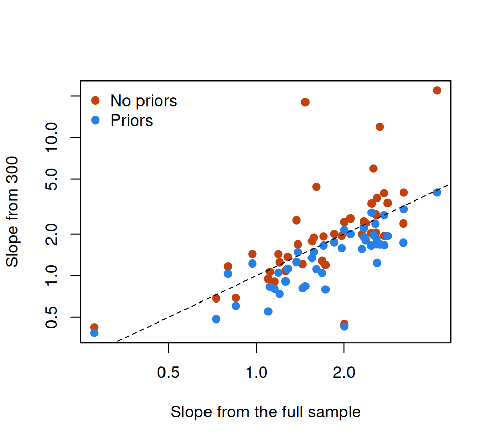
Fitted to 300 respondents without priors, the slopes have an SD of 4.15 and four exceed 5, while the full-sample slopes run from 0.28 to 4.16. With the priors, the SD is 0.75 and none exceeds 5, and the slopes’ error against the full-sample 3PL drops from 3.98 to 0.61. In this subsample the difficulties go the other way (0.80 to 1.12).
Code
# One subsample could be lucky. Five more, summarized by the median across them.
many <- sapply(2:6, function(s) compare(s)$summary)
round(apply(many, 1, median), 2)
sd_a_none sd_a_prior a_over_5_none a_over_5_prior rmse_a_none
2.30 0.77 3.00 0.00 2.11
rmse_a_prior rmse_b_none rmse_b_prior
0.76 5.62 2.84 Over five more subsamples (medians above) the priors again tame the slopes (error 2.11 against 0.76), and the difficulties improve too (5.62 against 2.84; on items nearly everyone gets right, a difficulty from 300 respondents can land almost anywhere). “Error” here is distance from the full-sample 3PL, not from the truth.
Problems
- What an answer is worth. With \(c\) fixed at \(1/k\), differentiate the log likelihood for \(\theta\) from one correct and from one incorrect response. Show that the first is smaller than under the Rasch model at every \(\theta\) and the second unchanged. What does that mean for a respondent who gets most items wrong?
- Real data with a twist. In
roar_lexical, set responses faster than 0.3 seconds to missing and refit the Rasch model and the fixed-floor model. How does the out-of-sample IMV change? - Real data: the items below chance. Refit both models without the 17
roar_lexicalitems answered correctly by fewer than half the respondents. What would a lower asymptote below 0.5 mean for those items? (PS4#3.) - Judgment (a live case). Fitted to all 2,802
vocabulary_iqrespondents who never chose “don’t know”, the 78 low scorers included, the 3PL puts every lower asymptote between 0.000 and 0.093, with a median of 0.000 (the output above). A colleague concludes that nobody guesses on this test. What would you check before agreeing? - Design. You must fit a 3PL to 200 respondents on a 30-item, four-option test. Choose priors, defend them, and check them by simulation. How would you know if your prior on \(c\) were in the wrong place? (PS4#4.)
- Challenge (open): guessing as a respondent trait. Compare the Rasch model, the fixed floor and the mixture on held-out
roar_lexicalresponses, by the IMV. Does the mixture’s in-sample gain survive? What would response times add? I don’t know of a single answer; Response time and the speed-accuracy tradeoff and Nominal response and multiple-choice models have pieces of one.
Going further
- Domingue, B. W., Kanopka, K., Kapoor, R., Pohl, S., Chalmers, R. P., Rahal, C., & Rhemtulla, M. (2024). The InterModel Vigorish as a lens for understanding (and quantifying) the value of item response models for dichotomously coded items. Psychometrika, 89(3), 1034–1054. https://doi.org/10.1007/s11336-024-09977-2. §3 and Table 1: how much the 3PL adds to prediction over the 2PL in simulation, including when it generated the data.
- Maris, G., & Bechger, T. (2009). On interpreting the model parameters for the three parameter logistic model. Measurement: Interdisciplinary Research and Perspectives, 7(2), 75–88. https://doi.org/10.1080/15366360903070385. What the 3PL’s parameters can and can’t be read as.
- von Davier, M. (2009). Is there need for the 3PL model? Guess what? Measurement: Interdisciplinary Research and Perspectives, 7(2), 110–114. https://doi.org/10.1080/15366360903117079. A commentary in the same issue.
- Haberman, S. J. (2005). Identifiability of parameters in item response models with unconstrained ability distributions. ETS Research Report Series, 2005(2), i–22. https://doi.org/10.1002/j.2333-8504.2005.tb02001.x. Identification in general form.
- Han, K. T. (2012). Fixing the c parameter in the three-parameter logistic model. Practical Assessment, Research, and Evaluation, 17, Article 1. https://doi.org/10.7275/f0gz-kc87. Fixing \(c = 1/k\), on simulated and real multiple-choice data.
- San Martín, E., del Pino, G., & De Boeck, P. (2006). IRT models for ability-based guessing. Applied Psychological Measurement, 30(3), 183–203. https://doi.org/10.1177/0146621605282773. Ways to add guessing to the 1PL, and a model in which the chance of a correct guess rises with ability.
- Xiao, X., Ulitzsch, E., Zhang, L., Frank, M. C., & Domingue, B. W. (2026). The safety valve: A mixture IRT approach to modeling guessing behavior. PsyArXiv preprint. https://doi.org/10.31234/osf.io/7gtwd_v1. The two-class mixture fitted to
roar_lexical, compared with the Rasch model and fixed floors by the IMV. - Schnipke, D. L., & Scrams, D. J. (1997). Modeling item response times with a two-state mixture model: A new method of measuring speededness. Journal of Educational Measurement, 34(3), 213–232. https://doi.org/10.1111/j.1745-3984.1997.tb00516.x. Rapid guesses and solution behaviour as two states.
- Wise, S. L., & Kong, X. (2005). Response time effort: A new measure of examinee motivation in computer-based tests. Applied Measurement in Education, 18(2), 163–183. https://doi.org/10.1207/s15324818ame1802_2. Engagement measured from response times.
- Wise, S. L. (2017). Rapid-guessing behavior: Its identification, interpretation, and implications. Educational Measurement: Issues and Practice, 36(4), 52–61. https://doi.org/10.1111/emip.12165. How rapid guesses are found, and what to do with them.
- Mislevy, R. J. (1986). Bayes modal estimation in item response models. Psychometrika, 51(2), 177–195. https://doi.org/10.1007/bf02293979. Priors on item parameters as well as abilities.
- Swaminathan, H., & Gifford, J. A. (1986). Bayesian estimation in the three-parameter logistic model. Psychometrika, 51(4), 589–601. https://doi.org/10.1007/BF02295598. Priors that keep 3PL estimates inside the parameter space.
- Harwell, M. R., & Baker, F. B. (1991). The use of prior distributions in marginalized Bayesian item parameter estimation: A didactic. Applied Psychological Measurement, 15(4), 375–389. https://doi.org/10.1177/014662169101500409. Mislevy’s procedure, step by step.
- Yeatman, J. D., Tang, K. A., Donnelly, P. M., Yablonski, M., Ramamurthy, M., Karipidis, I. I., Caffarra, S., Takada, M. E., Kanopka, K., Ben-Shachar, M., & Domingue, B. W. (2021). Rapid online assessment of reading ability. Scientific Reports, 11, 6396. https://doi.org/10.1038/s41598-021-85907-x. The lexical decision task behind
roar_lexical. - Chalmers, R. P. (2012). mirt: A multidimensional item response theory package for the R environment. Journal of Statistical Software, 48(6). https://doi.org/10.18637/jss.v048.i06. The package, including its
guessargument andPRIORsyntax. - From the IRW: the guessing vignette.
- Johnson, M. S., & Sinharay, S. (2017). Bayesian estimation. In W. J. van der Linden (Ed.), Handbook of item response theory: Vol. 2. Statistical tools (pp. 237–258). Chapman and Hall/CRC. https://doi.org/10.1201/b19166-13. A handbook chapter on Bayesian estimation for item response models.
- Sinharay, S. (2017). Bayesian model fit and model comparison. In W. J. van der Linden (Ed.), Handbook of item response theory: Vol. 2. Statistical tools (pp. 379–394). Chapman and Hall/CRC. https://doi.org/10.1201/b19166-19. A handbook chapter on Bayesian checks of model fit and Bayesian model comparison.
Data sources
Data from the Item Response Warehouse (each table name links to its IRW page); references from IRW biblio.
roar_lexical: Yeatman, J. D., Tang, K. A., Donnelly, P. M., Yablonski, M., Ramamurthy, M., Karipidis, I. I., … & Domingue, B. W. (2021). Rapid online assessment of reading ability. Scientific reports, 11(1), 6396. https://doi.org/10.1038/s41598-021-85907-x. Licence: CC BY 4.0.vocabulary_iq: (2018). Vocabulary IQ Test [dataset and codebook]. http://openpsychometrics.org/_rawdata/VIQT_data.zip. Licence: CC BY 4.0.
For instructors
- Source: EDUC 252 class 4 (slides c4, 33 and 60–61), problem set 4 (#3 and #4), and the code in
ben-domingue/252:ps4/guessing.R,ps4/priors.R. - Timing: the core ideas and widgets take about 50 minutes; the real-data section works as a 30-minute lab. Locally, the
roar_lexicalcross-validation takes a few minutes and thevocabulary_iqsubsamples several more; start them first. - Changed from 252: PS4#3 fixes guessing on the LEVANTE vocabulary task, which isn’t a tokenless IRW table; this lesson uses
roar_lexical, the alternative PS4#3’s code names, and adds the out-of-sample comparison (the PS4#3 bonus), the items below chance and the response times. PS4#4 puts priors on a 3PL forgilbert_meta_2; here they go onvocabulary_iqat 300 respondents, where they have more to do, and the design half of PS4#4 is problem 5. - Held back: response times modelled jointly with accuracy (Response time and the speed-accuracy tradeoff, which reuses
roar_lexical); skipped and “don’t know” responses as information (IRTree models); the wrong options (Nominal response and multiple-choice models); EM with priors on item parameters (Estimating item parameters). Deep dive #22 (which guessing correction helps across the IRW’s multiple-choice tables) is not built here. - Solutions: held back in
solutions/guessing-priors.qmd(not published).