Many sources of error: generalizability theory
What this is for
Classical test theory gives a score one error term. Suppose 202 people list unusual uses for a paperclip, a garbage bag and a rope, and five raters judge how clever each list is. A respondent might have done better with other objects, and would have got a different score from other raters. Which source of error is larger decides whether to add raters or objects. Generalizability theory (G theory) asks what the score should generalize over, then splits the error into those sources and prices each one (Cronbach, Rajaratnam & Gleser, 1963). In the cleverness ratings the answer is more tasks; in teachers’ ratings of essays, more raters. Like CTT, G theory is a theory of observed scores. Item response theory, from The Rasch model on, is a latent-trait theory that models each response, and the two rest on different assumptions.
Goals
By the end of this lesson you should be able to:
- name the facets of a measurement design, say which are crossed and which nested, and decide which the score should generalize over (random) and which not (fixed);
- estimate variance components for a persons × tasks × raters design with
lme4, and say which ones are error for which decision; - compute relative and absolute G coefficients, and show that the one-facet relative coefficient is alpha;
- use a D study to decide whether to add tasks or raters;
- compute consistency and agreement intraclass correlations, and say what each counts as error.
Core ideas
One error term, many sources
Where does \(E\) come from? The items behind alpha are one source; From construct map to items added another, the rater who scores a constructed response; occasions and forms are more. G theory calls each such source a facet, and each of its values (this rater, that task) a condition (Cronbach, Gleser, Nanda & Rajaratnam, 1972, a book with no DOI, linked here through Bock’s review in Science).
G theory applies that view to every facet. The tasks we used are a sample from the tasks we could have used; the raters, from the raters we would accept. Together these make up the universe of admissible observations, which the investigator, not the data, defines. A decision maker may care about only part of it (raters trained on this rubric, say); that part is the universe of generalization. A respondent’s average over it is the universe score, G theory’s counterpart of the true score, and the question of this lesson is how well an average over the few conditions we used stands in for it (Shavelson, Webb & Rowley, 1989). A facet we generalize over is random; a facet we don’t (these three objects and no others) is fixed, and what is specific to its conditions stops being error (Brennan, 2001).
Variance components
Take the cleverness design: every person \(p\) does every task \(t\), and every rater \(r\) rates every response, so all three are crossed. A rating is a sum of effects: \[X_{ptr} = \mu + \nu_p + \nu_t + \nu_r + \nu_{pt} + \nu_{pr} + \nu_{tr} + \nu_{ptr,e}.\] Each \(\nu\) is a random effect with mean zero and its own variance, and the effects are uncorrelated, so the variance of one rating splits into seven variance components, \(\sigma^2_p + \sigma^2_t + \dots + \sigma^2_{ptr,e}\) (Brennan, 2001). \(\sigma^2_p\) is how much people differ, the signal; \(\sigma^2_r\), how much raters differ in severity; \(\sigma^2_{pt}\), how much people’s standing changes from task to task; \(\sigma^2_{pr}\), raters disagreeing about who is better. The last term mixes the three-way interaction with whatever else the design can’t separate from it, hence the \(e\).
Not every design is crossed. If each essay is read by its own teachers, raters are nested within essays (\(r{:}p\)), and a teacher seen with one essay can’t show both how harsh they are and how they react to that essay: \(\sigma^2_r\) and \(\sigma^2_{pr}\) merge into \(\sigma^2_{r:p}\) (Brennan, 2001).
How do we estimate them? Classically, by setting the mean squares of an analysis of variance equal to their expected values, a reasonable choice for a balanced design (Brennan, 2001) and one the essay section uses as a check. This lesson fits each term as a random intercept in a mixed model, with lme4 (Bates, Mächler, Bolker & Walker, 2015) and a long table of one row per rating:
lmer(resp ~ 1 + (1 | id) + (1 | item) + (1 | rater) +
       (1 | id:item) + (1 | id:rater) + (1 | item:rater), data = ratings)
The residual variance is \(\sigma^2_{ptr,e}\). lmer estimates the variances by restricted maximum likelihood (REML). Plain maximum likelihood treats the fixed effects as known and so underestimates each variance, by more the fewer levels a facet has; REML removes that bias (Patterson & Thompson, 1971; Harville, 1977), which matters with facets of three and five levels. In a balanced design REML reproduces the ANOVA estimates whenever none is negative (Searle, Casella & McCulloch, 1992), and it also handles sparse designs like the second table’s.
Two G coefficients
Why are some components error only some of the time? It depends on the decision. For a relative decision (who ranks above whom), only the components that change a person’s standing count: those that interact with \(p\). For a score averaged over \(n_t\) tasks and \(n_r\) raters, the relative error variance is \[\sigma^2_\delta = \frac{\sigma^2_{pt}}{n_t} + \frac{\sigma^2_{pr}}{n_r} + \frac{\sigma^2_{ptr,e}}{n_t n_r}.\] For an absolute decision (is this score above 3? how clever is this list, on the rating scale?), a harsh rater or a hard task moves the score itself, so the main effects count too: \[\sigma^2_\Delta = \sigma^2_\delta + \frac{\sigma^2_t}{n_t} + \frac{\sigma^2_r}{n_r} + \frac{\sigma^2_{tr}}{n_t n_r}.\] Each coefficient sets the universe-score variance against one of them (Brennan, 2001): the generalizability coefficient \(E\rho^2 = \sigma^2_p/(\sigma^2_p + \sigma^2_\delta)\) and the dependability coefficient \(\Phi = \sigma^2_p/(\sigma^2_p + \sigma^2_\Delta)\). Since \(\sigma^2_\Delta \ge \sigma^2_\delta\), \(\Phi\) is never the larger. Error near a cut score is taken up in What does a score mean?.
Both have the form of reliability in Classical test theory and reliability, \(\sigma^2_T/(\sigma^2_T + \sigma^2_E)\): the “true” variance is universe-score variance, \(\sigma^2_p\), what stays with a person across the conditions we generalize over, and the error is what changes from one sample of conditions to another. Fix a facet and the split moves (the interrater section shows how).
Try it: the two coefficients side by side
Each bar is one coefficient’s denominator: the universe score plus the error it counts; the light pieces count only for Φ. The sliders start at the cleverness estimates from With real data; switch to the essays to see raters that differ in severity (there, “task” is a rating criterion).
The coefficients agree when raters and tasks don’t differ in harshness or difficulty (cleverness: 0.71 and 0.71) and part when they do (essays, one teacher: 0.47 and 0.40). The interrater section takes up which design each one describes.
What does the simplest case look like? Keep one facet, items, in a persons × items design. Then \(\sigma^2_\delta = \sigma^2_{pi,e}/n_i\) and \[E\rho^2 = \frac{\sigma^2_p}{\sigma^2_p + \sigma^2_{pi,e}/n_i},\] which is Cronbach’s alpha (Cronbach, 1951; Hoyt, 1941, estimated reliability from the same analysis of variance). The callout shows why.
D studies: what would another design buy?
A decision study (D study) uses the G study’s components to ask what a different design would give for the universe of generalization: which facets are random, and how many conditions of each are averaged over. Change \(n_t\) and \(n_r\) in the formulas and recompute. With one facet this is Spearman–Brown (problem 1); with two, the components say which lever moves the coefficient more.
Try it: a D study
The components are the ones set in the previous widget. Each line is a number of raters; the horizontal axis is the number of tasks.
With the cleverness components, ten tasks with one rater reach 0.74, one task with ten raters 0.49: person × task (0.284) dwarfs person × rater (0.053). Switch the previous widget to the essays and raters become the lever. Every curve flattens: past a point only the other facet helps.
What are we assuming when a D study adds raters we never had, ten when the data had five? That new raters are exchangeable draws from the universe of generalization, disagreeing with the others as much as the old ones did, and that the design stays crossed. Raters from a different pool change \(\sigma^2_r\) and \(\sigma^2_{pr}\); if each respondent gets different raters, severity joins the relative error (next section). And components estimated from a handful of raters make a far projection uncertain (Simulate shows how noisy a facet with three levels is).
Interrater reliability as a G study
In a persons × raters design, the setting for interrater reliability, the intraclass correlations of Shrout and Fleiss (1979) and McGraw and Wong (1996) are G coefficients. The consistency ICC for one rater, ICC(C,1) in McGraw and Wong’s notation, is \(\sigma^2_p/(\sigma^2_p + \sigma^2_{pr,e})\), the relative coefficient. The absolute agreement ICC, ICC(A,1), is \(\sigma^2_p/(\sigma^2_p + \sigma^2_r + \sigma^2_{pr,e})\), the dependability coefficient. Averaged over \(k\) raters, they are the D study for \(k\) raters.
When raters score the same tasks and the question is only whether another rater would score the same response the same way, the tasks are fixed. Brennan (2001) then puts \(\sigma^2_{pt}\) in the universe score: for one rater on one task the coefficient is \((\sigma^2_p + \sigma^2_{pt})/(\sigma^2_p + \sigma^2_{pt} + \sigma^2_{pr} + \sigma^2_{ptr,e})\), the answer to a narrower question than a coefficient that generalizes over tasks too.
Try it: consistency and agreement
Forty simulated respondents, two raters. Rater B is harsher by a constant; both add rating noise.
At the starting values consistency is 0.84 and agreement 0.62: the points lie along a line, below the dashed line of equal ratings. At harshness 0 the two meet; at 2 agreement falls to 0.35 while consistency stays at 0.84. Agreement charges for the gap.
Which coefficient describes the scores depends on the design and the use. If every respondent has the same raters and only the order matters, severity cancels. If scores are compared with a fixed standard, or respondents have different raters (each essay its own teachers, a nested design), a harsh rater lowers some scores and not others, and rater variance is error even for ranking (Brennan, 2001). In the case that raters vary across respondents or a cut is involved, the absolute coefficient, \(\Phi\) or the agreement ICC, may be the one to report; for a fully crossed design whose scores are used only to rank, the consistency coefficient may be sufficient for some purposes.
Simulate
The code generates a persons × tasks × raters design with known variance components (150 persons, 3 tasks, 3 raters, loosely like the cleverness ratings), fits the crossed model with lme4, and compares the estimates and G coefficients with the truth. Loading lme4 takes 10 to 20 seconds the first time the page runs code; the fit, about two.
With the seed as written, the person components come back close (person 0.346 against 0.30; person × task 0.317 against 0.30), and so does the relative coefficient (0.692 against 0.668). The task component does not (0.065 against 0.02): its variance is estimated from three numbers, however many persons there are. Set nt <- 10 and the coefficient rises to 0.842; put it back and set nr <- 10, and it rises only to 0.723.
With real data
Code
library(lme4)
options(digits = 7, scipen = 5)  # R's default digits, in case a .Rprofile changes it; no e-notation
# Variance components from a crossed random-effects fit, with their shares of the
# total. `labels` renames lme4's grouping factors (id, item, rater and their
# interactions) to the facets of the design.
components <- function(fit, labels) {
  vc <- as.data.frame(VarCorr(fit))
  v <- setNames(vc$vcov, labels[vc$grp])[labels]
  data.frame(variance = round(v, 3), percent = round(100 * v / sum(v), 1))
}
# G coefficients for a D study that averages over n_i levels of the first facet
# (tasks, or criteria) and n_r raters. v holds the seven components in the order
# p, i, r, pi, pr, ir, residual.
g_coef <- function(v, n_i, n_r) {
  rel <- v[4] / n_i + v[5] / n_r + v[7] / (n_i * n_r)
  abs <- rel + v[2] / n_i + v[3] / n_r + v[6] / (n_i * n_r)
  c(relative = v[1] / (v[1] + rel), absolute = v[1] / (v[1] + abs))
}
labels <- c(id = "person", item = "task", rater = "rater", "id:item" = "person x task",
            "id:rater" = "person x rater", "item:rater" = "task x rater",
            Residual = "residual (p x t x r, e)")
form <- resp ~ 1 + (1 | id) + (1 | item) + (1 | rater) +
  (1 | id:item) + (1 | id:rater) + (1 | item:rater)
Cleverness ratings: tasks or raters?
The main example is Forthmann-2024-cleverness_ratings, released by Forthmann and Myszkowski (2024) for a special issue of the Journal of Intelligence (CC BY 4.0; Forthmann et al., 2017, is an earlier analysis). Respondents listed unusual uses for three objects (the alternate uses task), and five raters rated each list for cleverness, stored as 1 to 5, higher meaning cleverer (Silvia et al., 2008, study the reliability of such ratings). Download the code; it needs lme4.
Code
url <- "https://redivis.com/api/v1/tables/datapages.item_response_warehouse_2:v22_0.Forthmann-2024-cleverness_ratings/rows?format=csv"
cl <- read.csv(url)[, c("id", "item", "rater", "resp")]
c(respondents = length(unique(cl$id)), tasks = length(unique(cl$item)),
  raters = length(unique(cl$rater)), ratings = nrow(cl),
  missing = length(unique(cl$id)) * 3 * 5 - nrow(cl))
respondents tasks raters ratings missing
202 3 5 3020 10 Code
table(cl$resp) # cleverness, 1 to 5; higher = cleverer
   1    2    3    4    5
 150  815 1115  760  180
Ten ratings are missing, all for one respondent; lmer handles the imbalance.
Code
fit_cl <- lmer(form, data = cl)
vc_cl <- components(fit_cl, labels)
vc_cl| variance | percent | |
|---|---|---|
| person | 0.310 | 32.1 |
| task | 0.000 | 0.0 |
| rater | 0.020 | 2.1 |
| person x task | 0.284 | 29.4 |
| person x rater | 0.053 | 5.5 |
| task x rater | 0.012 | 1.2 |
| residual (p x t x r, e) | 0.286 | 29.6 |
People differ (person, 32.1% of the variance of one rating), but person × task is nearly as large (29.4%): being clever with a rope says only so much about being clever with a paperclip. Raters account for little: 2.1% for severity and 5.5% for disagreement about who is cleverer. The task component is estimated at zero, so the three objects are about equally hard to be clever with. How much did REML matter? Refit by plain maximum likelihood:
Code
# REML against plain maximum likelihood, for the two facets with few levels.
fit_ml <- lmer(form, data = cl, REML = FALSE)   # warns of a singular fit: task is 0
facet_var <- function(fit) {
  v <- as.data.frame(VarCorr(fit))
  setNames(v$vcov, v$grp)[c("item", "rater")]
}
round(rbind(REML = facet_var(fit_cl), ML = facet_var(fit_ml)), 4)   # item = task
item rater
REML 0.0004 0.0199
ML 0.0000 0.0163With five raters, maximum likelihood puts rater severity at about four-fifths of the REML value, the downward bias REML removes.
Code
v_cl <- vc_cl$variance
round(g_coef(v_cl, 3, 5), 2)     # the design as run: 3 tasks, 5 raters
relative absolute
0.71 0.71 Code
round(g_coef(v_cl, 3, 1), 2) # 3 tasks, 1 raterrelative absolute
0.56 0.54 Code
round(g_coef(v_cl, 6, 1), 2) # 6 tasks, 1 raterrelative absolute
0.68 0.65 Code
round(g_coef(v_cl, 3, 1e6), 2) # 3 tasks, as many raters as you likerelative absolute
0.77 0.77 Code
d_grid <- expand.grid(tasks = 1:10, raters = c(1, 2, 5))
d_grid$relative <- mapply(function(t, r) g_coef(v_cl, t, r)[1], d_grid$tasks, d_grid$raters)
Code
cols <- c("1" = "#93c5fd", "2" = "#2780e3", "5" = "#c2410c")
plot(NULL, xlim = c(1, 10), ylim = c(0, 1), xlab = "Tasks averaged over",
     ylab = "Relative G coefficient", las = 1, main = "Cleverness ratings: a D study")
for (r in c(1, 2, 5)) with(d_grid[d_grid$raters == r, ],
                           lines(tasks, relative, type = "b", pch = 19, lwd = 2, col = cols[as.character(r)]))
abline(h = 0.8, col = "#999", lty = 2)
legend("bottomright", paste(c(1, 2, 5), c("rater", "raters", "raters")), col = cols,
       lwd = 2, pch = 19, bty = "n")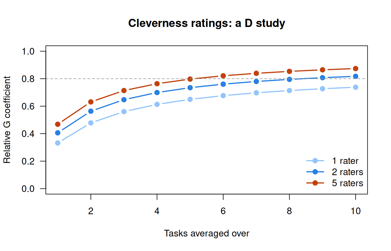
The design as run, 3 tasks and 5 raters, has a relative G coefficient of 0.71. One rater gives 0.56, but one rater with 6 tasks gives 0.68: 6 ratings per respondent instead of 15, for nearly the same coefficient. No number of raters takes 3 tasks past 0.77, the ceiling set by person × task. For this construct and these raters, adding tasks buys more than adding raters. The absolute coefficient equals the relative one to two decimals (0.71), since the task and rater components are small.
If the tasks are fixed instead, as in the interrater coefficient of Brennan (2001), person × task joins the universe score:
Code
# Interrater reliability with the tasks fixed: raters score the same tasks, so the
# person x task effect is part of the universe score. One rater, one task:
round(c(tasks_fixed = (v_cl[1] + v_cl[4]) / (v_cl[1] + v_cl[4] + v_cl[5] + v_cl[7]),
        tasks_random = unname(g_coef(v_cl, 1, 1)[1])), 2)
tasks_fixed tasks_random
0.64 0.33 A second rater would score the same list much as the first did (0.64), but a respondent’s cleverness with one object says much less about their cleverness in general (0.33). Same ratings, two universes.
Essays: when raters matter
The contrast is teacherjudgements_lohmann_2026_essayratings, from a study in which preservice English teachers rated essays by learners of English as a second language (Lohmann et al., 2026; CC BY 4.0). Each teacher rated five essays on four criteria (language quality, structure, content, and a holistic rating), from 1 (very low quality) to 7 (very high quality). “Person” in the output now means essay, and criteria take the place of tasks. We set aside the table’s expert benchmark scores.
Code
url <- "https://redivis.com/api/v1/tables/datapages.item_response_warehouse_4:v7_0.teacherjudgements_lohmann_2026_essayratings/rows?format=csv"
es <- read.csv(url)
# The table also holds an expert benchmark score for every essay and criterion;
# the G study is about the teachers, so set it aside.
es <- es[es$rater != "expert_benchmark", c("id", "item", "rater", "resp")]
c(essays = length(unique(es$id)), criteria = length(unique(es$item)),
  teachers = length(unique(es$rater)), ratings = nrow(es))
essays criteria teachers ratings
881 4 315 6300 Code
table(es$resp) # 1 (very low quality) to 7 (very high quality)
   1    2    3    4    5    6    7
 280  842 1142 1383 1310  948  395
Code
pairs <- unique(es[, c("id", "rater")])
table(table(pairs$rater))   # essays per teacher
  5
315
Code
table(table(pairs$id)) # teachers per essay
  1   2   3   4   5   6   7
435 270 126  34  11   4   1
This design is sparse. Every teacher rated 5 essays, but 435 of the 881 essays were rated by a single teacher, and only 50 by four or more. Each essay has its own teachers, so raters are effectively nested within essays, though each teacher’s five essays link the teachers to one another.
How does the fit handle the essay–teacher pairs never observed? Nothing is filled in. REML uses only the ratings that exist and learns each component where ratings overlap: a teacher’s severity from how their five essays fare against other ratings of those essays, essay × rater from essays that two or more teachers read, essay × criterion from the four criteria of every rating. An essay read by one teacher informs the essay and criterion components but can’t, alone, separate that teacher’s view of it from the essay itself.
Code
# The default optimizer stops just short of lme4's convergence tolerance on this
# fit; bobyqa converges and gives the same estimates to three decimals.
fit_es <- lmer(form, data = es, control = lmerControl(optimizer = "bobyqa"))
vc_es <- components(fit_es, sub("t x r", "c x r", sub("task", "criterion", labels)))
vc_es| variance | percent | |
|---|---|---|
| person | 0.754 | 29.7 |
| criterion | 0.010 | 0.4 |
| rater | 0.246 | 9.7 |
| person x criterion | 0.243 | 9.6 |
| person x rater | 0.640 | 25.2 |
| criterion x rater | 0.047 | 1.8 |
| residual (p x c x r, e) | 0.602 | 23.7 |
The picture reverses. Teachers differ in severity (rater, 9.7% of the variance, against 2.1% in the cleverness ratings), and essay × rater is 25.2%, against the essays’ own 29.7%: teachers disagree about which essays are better. Criteria matter less (essay × criterion, 9.6%). Since each teacher rated an essay on all four criteria, essay × rater is an impression that carries across them, the pattern a halo effect (named in Lohmann et al.’s title) would produce. Teachers’ severity has an SD of 0.50 points, against 0.87 for essays’ universe scores.
Code
v_es <- vc_es$variance
sapply(c(1, 2, 3, 5), function(r) round(g_coef(v_es, 4, r), 2))   # 4 criteria, 1-5 raters
[,1] [,2] [,3] [,4]
relative 0.47 0.62 0.70 0.78
absolute 0.40 0.56 0.65 0.73Code
round(g_coef(v_es, 1e6, 1), 2) # one rater, as many criteria as you likerelative absolute
0.54 0.46 Code
round(sqrt(v_es[c(1, 3)]), 2) # SD of essays' universe scores; SD of teachers' severity[1] 0.87 0.50With one teacher and four criteria, the relative coefficient is 0.47 and the absolute 0.40. A second teacher brings them to 0.62 and 0.56; five, to 0.78 and 0.73. One teacher on unlimited criteria reaches only 0.54: the lever is raters. Since each essay had its own teachers, the absolute coefficient describes these scores.
A check: the balanced subset
Is the sparse fit believable? Part of the data is balanced: the essays rated by exactly three teachers, each on all four criteria.
Code
# A balanced part of the essay data: the essays rated by exactly three teachers,
# each on all four criteria. Treating each essay's teachers as its own (raters
# nested within essays) makes the design (r:p) x c, the classic balanced case.
n_teach <- table(pairs$id)
bal <- es[es$id %in% names(n_teach)[n_teach == 3], ]
c(essays = length(unique(bal$id)), teachers = length(unique(bal$rater)), ratings = nrow(bal))
essays teachers ratings
126 241 1512 Code
table(table(bal$id)) # ratings per essay: 3 teachers x 4 criteria = 12 for every essay
 12
126
Treating each essay’s teachers as its own gives the design \((r{:}p) \times t\) (criteria as \(t\)), with five components: essay, criterion, rater within essay, essay × criterion and the residual. The classic route works here: compute the mean squares and solve the expected-mean-squares equations (the callout gives them).
Code
# The classic route, by hand: sums of squares, mean squares, then the
# expected-mean-squares equations solved for the five components (see the callout).
# ave() returns each row's group mean, so the sums run over all ratings.
n_p <- length(unique(bal$id)); n_r <- 3; n_c <- 4
m    <- mean(bal$resp)
m_p  <- ave(bal$resp, bal$id)                 # essay means
m_c  <- ave(bal$resp, bal$item)               # criterion means
m_rp <- ave(bal$resp, bal$id, bal$rater)      # teacher-within-essay means
m_pc <- ave(bal$resp, bal$id, bal$item)       # essay x criterion means
ss <- c(p = sum((m_p - m)^2), c = sum((m_c - m)^2), "r:p" = sum((m_rp - m_p)^2),
        pc = sum((m_pc - m_p - m_c + m)^2), "rc:p,e" = sum((bal$resp - m_rp - m_pc + m_p)^2))
df <- c(n_p - 1, n_c - 1, n_p * (n_r - 1), (n_p - 1) * (n_c - 1), n_p * (n_r - 1) * (n_c - 1))
ms <- ss / df
round(cbind(df, ms), 3)
df ms
p 125 14.251
c 3 10.110
r:p 252 4.205
pc 375 1.340
rc:p,e 756 0.597Code
v_anova <- c(essay = (ms[["p"]] - ms[["r:p"]] - ms[["pc"]] + ms[["rc:p,e"]]) / (n_r * n_c),
             criterion = (ms[["c"]] - ms[["pc"]]) / (n_p * n_r),
             "rater within essay" = (ms[["r:p"]] - ms[["rc:p,e"]]) / n_c,
             "essay x criterion" = (ms[["pc"]] - ms[["rc:p,e"]]) / n_r,
residual = ms[["rc:p,e"]])Now the same design by REML, next to the full sparse fit with its components combined to match (rater within essay is rater plus essay × rater; the residual absorbs criterion × rater):
Code
# The same design by REML: id:rater is a teacher within an essay.
fit_bal <- lmer(resp ~ 1 + (1 | id) + (1 | item) + (1 | id:rater) + (1 | id:item), data = bal)
vb <- as.data.frame(VarCorr(fit_bal))
v_reml <- setNames(vb$vcov, vb$grp)[c("id", "item", "id:rater", "id:item", "Residual")]
# The full sparse fit, its seven components combined to match the nested design:
# rater within essay = rater + essay x rater; residual = criterion x rater + residual.
vf <- as.data.frame(VarCorr(fit_es))
vf <- setNames(vf$vcov, vf$grp)
v_full <- c(vf[["id"]], vf[["item"]], vf[["rater"]] + vf[["id:rater"]], vf[["id:item"]],
            vf[["item:rater"]] + vf[["Residual"]])
round(cbind(ANOVA = v_anova, REML = v_reml, "full sparse fit" = v_full), 3)
ANOVA REML full sparse fit
essay 0.775 0.775 0.754
criterion 0.023 0.023 0.010
rater within essay 0.902 0.902 0.886
essay x criterion 0.248 0.248 0.243
residual 0.597 0.597 0.648Code
signif(max(abs(v_anova - v_reml)), 2) # largest gap between ANOVA and REML[1] 0.000014ANOVA and REML agree to the third decimal: in a balanced design with no negative estimate, REML is the ANOVA solution. The full sparse fit is close: essay 0.754 against 0.775, rater within essay 0.886 against 0.902, residual 0.648 against 0.597. The gaps have three sources: a different set of essays (126 of 881, picked by how many teachers they got); a small sample, so noisy estimates (criterion, from four levels, most of all: 0.010 against 0.023); and a design that can’t split rater within essay into severity and essay × rater, as the full fit can. Where the data allow the classical estimate, REML on the sparse design gives much the same answer.
The two tables call for different designs, and only their variance components could say so.
Problems
- Derivation. Fill in the sums of squares in the Go deeper callout to show that \(1 - MS_{pi,e}/MS_p\) is alpha. Then show that the D-study coefficient for \(m n_i\) items is the Spearman–Brown formula with multiplier \(m\).
- Real data with a twist. From the cleverness components, find the combinations of tasks and raters that give a relative G coefficient of at least 0.8. Is there more than one? If a task costs a respondent five minutes and a rating costs a rater one minute per respondent, which design is cheapest for 200 respondents? Does the answer change for \(\Phi\)?
- Judgment: a sparse design. Refit the essay model using only essays with at least two teachers. Which components change, and how do they compare with the balanced subset’s? Suppose every essay had one teacher: which components could the data no longer separate, and what would that do to your D study?
- Design. Plan a G study for a performance assessment you know. What should the score generalize over? Name the facets, random or fixed, crossed or nested, and choose sample sizes. Which component do you expect to be largest?
- Real data: two raters. In the cleverness data, take raters 1 and 2 and the paperclip task. Compute the consistency and agreement ICCs from a
lmerfit with random intercepts for respondent and rater. Which pair of raters agrees least? - Challenge (open). G theory treats a harsh rater as a random effect to be averaged away. When should severity be estimated and adjusted for instead, and what would you need to know about the essays’ teachers to decide? (Rater models takes this up with the many-facet Rasch model.)
Going further
- Shavelson, R. J., & Webb, N. M. (1991). Generalizability theory: A primer. Sage. No DOI; see Sundre’s (1993) review. The most accessible first read, at book length.
- Brennan, R. L. (2001). Generalizability theory. Springer. https://doi.org/10.1007/978-1-4757-3456-0. The reference: designs, nested and fixed facets, estimation and D studies, at book length.
- Shavelson, R. J., Webb, N. M., & Rowley, G. L. (1989). Generalizability theory. American Psychologist, 44(6), 922–932. https://doi.org/10.1037/0003-066X.44.6.922. A short overview.
- Brennan, R. L. (2000). Performance assessments from the perspective of generalizability theory. Applied Psychological Measurement, 24(4), 339–353. https://doi.org/10.1177/01466210022031796. Which facets matter for performance assessments, and how popular reliability estimates for them, interrater reliability among them, look from G theory.
- Brennan, R. L. (1992). Generalizability theory. Educational Measurement: Issues and Practice, 11(4), 27–34. https://doi.org/10.1111/j.1745-3992.1992.tb00260.x. An instructional module on G and D studies.
- Cronbach, L. J., Gleser, G. C., Nanda, H., & Rajaratnam, N. (1972). The dependability of behavioral measurements: Theory of generalizability for scores and profiles. Wiley. No DOI; see Bock’s (1972) review. The book-length statement of the theory.
- Cronbach, L. J., Rajaratnam, N., & Gleser, G. C. (1963). Theory of generalizability: A liberalization of reliability theory. British Journal of Statistical Psychology, 16(2), 137–163. https://doi.org/10.1111/j.2044-8317.1963.tb00206.x. Where the theory starts.
- McGraw, K. O., & Wong, S. P. (1996). Forming inferences about some intraclass correlation coefficients. Psychological Methods, 1(1), 30–46. https://doi.org/10.1037/1082-989X.1.1.30. The ICCs, sorted by design and by consistency versus agreement.
- Bates, D., Mächler, M., Bolker, B., & Walker, S. (2015). Fitting linear mixed-effects models using lme4. Journal of Statistical Software, 67(1). https://doi.org/10.18637/jss.v067.i01. How
lmerspecifies and fits crossed random effects. - Eckes, T. (2011). Introduction to many-facet Rasch measurement. Peter Lang. https://doi.org/10.3726/978-3-653-04844-5. Raters as a facet in an item response model, which estimates each rater’s severity and adjusts scores for it; Rater models develops it on this lesson’s two tables.
- De Boeck, P. (2008). Random item IRT models. Psychometrika, 73(4), 533–559. https://doi.org/10.1007/s11336-008-9092-x. Items as random effects in an item response model, an idea What is an item? takes further.
Data sources
Data from the Item Response Warehouse (each table name links to its IRW page); references from IRW biblio.
Forthmann-2024-cleverness_ratings: Forthmann, Boris, and Nils Myszkowski. 2024. “Analysis of a Divergent Thinking Dataset.” OSF. April 22. osf.io/a9qnc. <https://doi.org/No DOI>. Licence: CC BY 4.0.teacherjudgements_lohmann_2026_essayratings: Lohmann, J. F., Lötscher, F., Junge, F., Keller, S., Jansen, T., Fleckenstein, J., & Möller, J. (2026). Testing teacher judgments comprehensively: Accuracy, halo, frame of reference, strategy, and personality effects in holistic and analytic assessments of student essays.Journal of Educational Psychology, 118(6), 941–960. https://doi.org/10.1037/edu0000969. Licence: CC BY 4.0.
For instructors
- Source: new material, not in EDUC 252. The course’s landscape analysis (
notes/landscape-2026-09-24.md, gap 2) put G theory and interrater reliability into one lesson. - Estimation (#76): the main line estimates variance components with
lme4(REML); the ANOVA / expected-mean-squares route appears twice, in the Go deeper on alpha and in the balanced essay subset, where it matches REML. Comments on #76 asked for what the score generalizes over, the assumptions behind D-study projections, Brennan’s interrater coefficient with tasks fixed, observed-score versus latent-trait theories, the universe of generalization, crossed versus nested designs, and how the sparse essay design is handled; those are in this version. - Timing: about 50 minutes for the core ideas and widgets; the two real-data analyses work as a 25-minute lab (the essay fit takes about half a minute in local R).
- Held back: nested designs appear only in the balanced essay subset, and fixed facets only in the interrater coefficient (see Shavelson & Webb, 1991, and Brennan, 2001); multivariate G theory is not covered. Raters in item response models (many-facet Rasch) are left to Rater models; random item effects to What is an item?; error near a cut to What does a score mean?; occasions as a facet to Measurement invariance under treatment and life events.
- Solutions: held back in
solutions/g-theory.qmd(not published). Problem 6 is open.