Factor analysis I: exploring dimensionality
What this is for
How many things does a set of items measure? Classical test theory mostly assumes the answer is one, and a high alpha doesn’t check that assumption. Many instruments are built to measure several things at once: a personality inventory with five domains, a quality-of-life scale with physical and emotional subscales. And an instrument meant to measure one thing may not, as the reverse-worded items in the instrument-building lesson showed. Factor analysis is the family of tools for asking what, and how many, underlying dimensions account for the correlations among a set of items. It is one of the oldest ideas in psychometrics. Spearman (1904) proposed it to explain why children who did well in one school subject tended to do well in others, and it remains the workhorse for studying the internal structure of a scale.
This lesson is about the exploratory version: we let the data suggest a structure. Factor analysis II takes up the confirmatory version, where we state a structure in advance and test it, and shows that factor analysis and item response theory are closer relatives than they first appear.
Goals
By the end of this lesson you should be able to:
- write down the common factor model and explain how it reproduces a correlation matrix;
- decide how many factors to extract, using eigenvalues and parallel analysis, and explain why common rules of thumb disagree;
- explain what rotation does (and what it does not do) and choose between orthogonal and oblique rotations;
- say why Likert items call for polychoric correlations, and how factor analysis differs from principal components;
- run an exploratory factor analysis on real item responses and read the output.
Core ideas
A model for correlations
The data for factor analysis is a correlation matrix. The common factor model says that each standardized item \(x_i\) is a weighted combination of a small number of common factors plus something unique to that item: \[x_i = \lambda_{i1} f_1 + \lambda_{i2} f_2 + \dots + \lambda_{im} f_m + u_i.\] The weights \(\lambda\) are the loadings. The unique part \(u_i\) bundles measurement error with anything specific to the item, and it is assumed to be uncorrelated with the factors and with the other items’ unique parts. That last assumption carries the model: it says that everything the items have in common runs through the factors. Spearman’s version had one factor; Thurstone (1931) extended it to several, and his Multiple-factor analysis (Thurstone, 1947; see the review by Cattell, 1948) set out most of what follows.
With a single factor, the model makes a strong prediction. The correlation between items \(i\) and \(j\) is just the product of their loadings, \[\text{cor}(x_i, x_j) = \lambda_i \lambda_j,\] so an entire matrix of correlations is generated by one loading per item. Try it.
Try it: correlations from one factor
You should see two things. The item with the weakest loading has the weakest correlations with everything. And the pattern is rigid: the ratio of item 1’s correlations with items 3 and 4 is the same as the ratio of item 2’s. If real data didn’t have that rigid pattern, one factor would not be enough, which is how factor analysis detects that a second dimension is needed. Spearman turned the rigid pattern into a test, the vanishing “tetrad differences” (Spearman & Holzinger, 1924; problem 1).
A useful quantity falls out of this: an item’s communality, \(h_i^2 = \sum_k \lambda_{ik}^2\), is the share of its variance explained by the common factors. The remainder, \(1 - h_i^2\), is its uniqueness. An item with loading 0.3 on a single factor has a communality of \(0.3^2 = 0.09\); more than 90% of what it does is its own business.
A one-factor model is what “the items are unidimensional” means in factor-analytic terms, and it is a claim the data can reject.
How many factors?
This is the question exploratory factor analysis is most often used to answer, and it has no single correct procedure. The usual starting point is the eigenvalues of the correlation matrix. Loosely, each eigenvalue says how much of the total variance (which, for \(p\) standardized items, is \(p\)) a dimension can account for, taken in decreasing order. A few large eigenvalues followed by a flat tail suggests a few factors.
Two classic rules of thumb read this list. The Kaiser rule keeps every factor with an eigenvalue above 1 (Guttman, 1954; Kaiser, 1960). The scree plot looks for the “elbow” where the eigenvalues level off (Cattell, 1966). Both have a problem: even data with no factor structure produce eigenvalues above 1, purely from sampling variability, and more so in small samples. Parallel analysis (Horn, 1965) fixes this by comparing the observed eigenvalues with those from random data of the same size, and keeping factors only while the observed ones are larger. It asks a narrower question than it may seem to: whether a dimension stands out from sampling noise, not whether it means anything.
Try it: eigenvalues and parallel analysis
Twelve items, generated from a known number of factors.
At the starting settings (two factors, loadings of 0.5, 150 people), parallel analysis finds two factors and the Kaiser rule four. Raise the sample to 500 and both find two: with loadings of 0.5 and 500 people, the Kaiser rule is a reasonable quick first look. Now drop the loadings to 0.3: the Kaiser rule says four or five even with 1,000 people, and with 100 people parallel analysis goes wrong too, in either direction depending on the number of factors. The number of factors is an estimate, with its own uncertainty, and the choice should also make substantive sense.
Rotation
Once we have more than one factor, which set of loadings is the right one? The data cannot say. With two or more factors the loadings are not unique: any rotation of the factors reproduces the correlation matrix exactly as well as any other. What rotation does is pick, from this infinite family of equally good solutions, one that is easy to interpret, ideally one with simple structure (Thurstone, 1947), where each item loads strongly on one factor and near zero on the rest.
Try it: rotating two factors
Six items, with the true loadings shown when the angle is 0. Rotate the factors and watch the loadings change while the fit does not.
The points swing around the origin as a rigid body, and the implied correlations never change. Only the simplicity score moves, and it is largest near an angle of 0, where each item sits close to one axis.
Rotations come in two kinds (Browne, 2001, reviews both). Orthogonal rotations keep the factors uncorrelated; varimax (Kaiser, 1958) is the best known. Oblique rotations let them correlate: oblimin (in R’s default form, direct quartimin; Jennrich & Sampson, 1966), promax (Hendrickson & White, 1964) and others. In psychology and education, constructs tend to correlate with one another, so forcing factors to be uncorrelated is an assumption we seldom have reason to make; an oblique rotation estimates the correlations instead of fixing them at zero. If the factors turn out to be nearly uncorrelated, the two approaches will agree anyway, and we’ll see below how far from zero the BFI-2’s factor correlations sit.
Two practical notes
Likert items are not continuous. Pearson correlations between 5-point items understate the relationship between the underlying continuous tendencies, and they are distorted when items are skewed. The standard fix is to factor-analyze polychoric correlations (Olsson, 1979), which estimate the correlation between the continuous variables that the ordered categories are assumed to coarsen. We use them below. This idea, an ordered response as a coarsened continuous one, is also the bridge to item response theory; see Factor analysis II.
Factor analysis is not principal components analysis. PCA (Pearson, 1901; Hotelling, 1933) finds weighted sums of the items that capture as much of their total variance as possible; it has no unique parts and no model of measurement error. Factor analysis models only the shared variance. For summarizing data the two often look similar (Velicer & Jackson, 1990); for asking what constructs an instrument measures, the separation of shared from unique variance is what factor analysis adds, and it is the reason Fabrigar et al. (1999) give for using it there. Problem 6 compares the two on real data.
Simulate
The code below builds a questionnaire with a known structure (by default, two correlated factors with five items each), runs parallel analysis, fits an oblique exploratory factor analysis, and prints the loadings for comparison with the truth. It uses the psych package (Revelle, 2026), with rotations from GPArotation (Bernaards & Jennrich, 2005), and estimates by minimum residuals (Harman & Jones, 1966). It runs in your browser; the first run takes a little while as psych loads.
Things to try: set loading to 0.4 or np to 100 and see whether parallel analysis still finds the right number of factors; set phi to 0.7 and ask whether two factors are still worth distinguishing; set n_factors to 3.
With the seed as written, the estimated factor correlation comes out at 0.18 against a true 0.3. That is sampling variability with 400 people, and a reminder that factor correlations are estimated with less precision than loadings. Download this code.
With real data
We use bfi2_zhang_2025, our main example: responses from 1,335 university students to the 60-item Big Five Inventory-2 (BFI-2; Soto & John, 2017), which measures five broad domains of personality with 12 items each. The data come from Zhang, Huang, Sun and Savalei (2025), who randomly assigned students to one of four response formats; we pool across formats here and return to that design in problem 4. Download the code.
Code
library(psych)
# Each IRW table has a landing page (itemresponsewarehouse.org/tables/<name>/)
# with a CSV download. This link is pinned to one version of the data.
url <- "https://redivis.com/api/v1/tables/datapages.item_response_warehouse_2:v21_0.bfi2_zhang_2025/rows?format=csv"
df <- read.csv(url)
wide <- tapply(df$resp, list(df$id, df$item), function(x) x[1])
num <- as.integer(sub("self_BFI_", "", colnames(wide)))
resp <- as.data.frame(wide[, order(num)])
c(respondents = nrow(resp), items = ncol(resp))
respondents items
1335 60 Code
resp <- resp[complete.cases(resp), ]
nrow(resp)   # respondents who answered all 60 items
[1] 1199A few responses are missing, scattered across items and respondents; we keep the 1,199 students who answered all 60.
Code
# The BFI-2 cycles through its five domains: item 1 is Extraversion, item 2
# Agreeableness, item 3 Conscientiousness, item 4 Negative Emotionality, item 5
# Open-Mindedness, item 6 Extraversion again, and so on (Soto & John, 2017).
domain <- c("Extraversion", "Agreeableness", "Conscientiousness",
            "Negative Emotionality", "Open-Mindedness")[(seq_len(60) - 1) %% 5 + 1]
table(domain)
domain
Agreeableness Conscientiousness Extraversion
12 12 12
Negative Emotionality Open-Mindedness
12 12 Responses run from 1 to 5, and they arrive keyed: the BFI-2’s reverse-worded items have already been reversed, so a higher response always means more of the item’s domain (for Negative Emotionality, more negative emotion). Neither the table’s metadata nor its processing code says so, and the data can only suggest it. If the reverse-worded items were still raw, many pairs of items from the same domain would correlate negatively. The lowest of these correlations is essentially zero:
Code
# Are the reverse-worded items already reversed? If they weren't, many pairs of
# items from the same domain would correlate clearly negatively.
r <- cor(resp)
same <- outer(domain, domain, "==") & lower.tri(r)
round(range(r[same]), 3)   # Pearson correlations between items of the same domain
[1] -0.005 0.764The correlation matrix
Before fitting anything, look at the correlations with the items sorted by the domain they were written for.
Code
# Polychoric correlations treat each 1-5 response as a coarsened continuous one.
R <- polychoric(resp)$rho
by_domain <- order(domain)
image(1:60, 1:60, R[by_domain, rev(by_domain)], zlim = c(-1, 1), axes = FALSE,
      col = hcl.colors(41, "Blue-Red 3"), xlab = "Items, grouped by domain", ylab = "",
      main = "Polychoric correlations, BFI-2 items sorted by domain")
abline(v = seq(12.5, 48.5, 12), h = seq(12.5, 48.5, 12), col = "white", lwd = 2)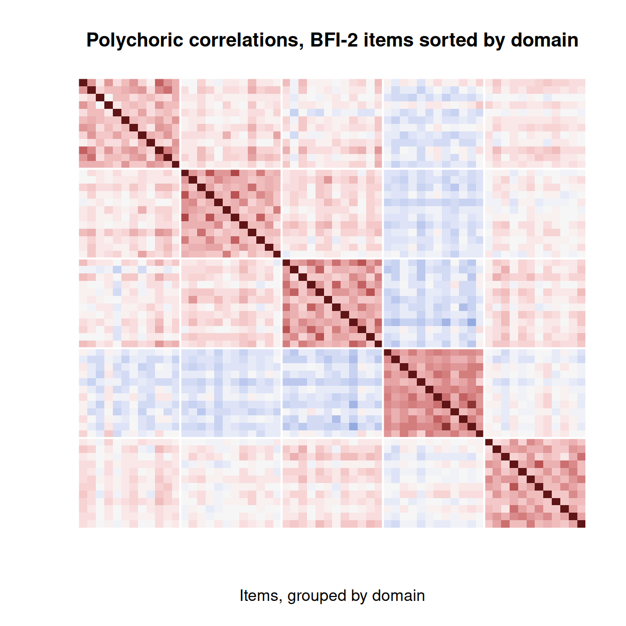
Code
off <- lower.tri(R)
round(c(within_domain = median(R[off & outer(domain, domain, "==")]),
        between_domains = median(R[off & outer(domain, domain, "!=")])), 2)
within_domain between_domains
0.35 0.04 Five blocks along the diagonal, and pale regions between them: the median correlation is 0.35 between two items of the same domain and 0.04 between items of different domains. The one band of blue belongs to Negative Emotionality (the fourth block, since the domains are sorted alphabetically), whose items correlate weakly and negatively with many of the others.
Do the BFI-2’s items also split by wording, as the Rosenberg items did? Half of each domain’s items are worded in reverse (the scoring key of Soto & John, 2017), so we can compare pairs of items worded in the same direction with pairs worded in opposite directions.
Code
# Reverse-worded items, from the BFI-2 scoring key (Soto & John, 2017). They arrive
# already reversed; here we only ask whether items worded in the same direction
# correlate more than items worded in opposite directions.
reversed <- seq_len(60) %in% c(3, 4, 5, 8, 9, 11, 12, 16, 17, 22, 23, 24, 25, 26, 28,
                               29, 30, 31, 36, 37, 42, 44, 45, 47, 48, 49, 50, 51, 55, 58)
same_dom <- outer(domain, domain, "==")
same_dir <- outer(reversed, reversed, "==")
round(c(same_domain_same_direction = median(R[off & same_dom & same_dir]),
        same_domain_opposite       = median(R[off & same_dom & !same_dir]),
        other_domain_same_direction = median(R[off & !same_dom & same_dir]),
        other_domain_opposite       = median(R[off & !same_dom & !same_dir])), 2)
same_domain_same_direction same_domain_opposite
0.35 0.35
other_domain_same_direction other_domain_opposite
0.05 0.02 Within a domain the two kinds of pair correlate equally, with a median of 0.35 each. Between domains, pairs worded the same way correlate 0.05 and pairs worded oppositely 0.02. By this measure wording direction leaves at most a trace in the BFI-2, far from the Rosenberg scale’s blocks.
How many factors?
Code
set.seed(252)
pa <- fa.parallel(R, n.obs = nrow(resp), fa = "fa", n.iter = 20, plot = TRUE,
                  main = "Parallel analysis: BFI-2")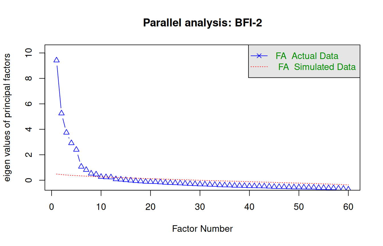
Parallel analysis suggests that the number of factors = 9 and the number of components = NA Code
ev <- eigen(R)$values
c(parallel = pa$nfact,
  kaiser = sum(ev > 1))           # the "eigenvalue greater than one" rule, for comparison
parallel kaiser
9 12 Code
round(ev[1] / ev[2], 2) # ratio of the first to the second eigenvalue[1] 1.67Code
# The same parallel analysis on Pearson correlations, for comparison:
set.seed(252)
fa.parallel(r, n.obs = nrow(resp), fa = "fa", n.iter = 20, plot = FALSE)$nfact
Parallel analysis suggests that the number of factors = 9 and the number of components = NA [1] 9Parallel analysis says 9, the Kaiser rule 12, against a design of five domains and 15 facets. Is that unusual? Across the IRW it is the norm. The IRW’s dimensionality vignette ran parallel analysis on 810 tables and found exactly one factor in only 3% of them; for the older 25-item Big Five Inventory in psychtools_bfi, built for five traits, it suggests six. Nor is it an artifact of the polychoric correlations, which Garrido, Abad and Ponsoda (2013) recommend for parallel analysis with ordinal items: on Pearson correlations the answer is 9 again. The formal criteria find more structure than the design names, because each domain is itself made of related facets.
The same vignette gives a baseline for how multidimensional the BFI-2 is. The ratio of the first to the second eigenvalue, 1.7 here, is a rough index of how far a scale is from a single dimension (larger means closer to one). The vignette’s 57 personality tables have a median ratio of 3.26, and the 25-item BFI’s is 1.91. The vignette’s tables have at most 40 items, so the comparison is rough, but by the IRW’s standard the BFI-2 is clearly multidimensional, as it was built to be.
The five-domain structure is still the one the instrument is built to score, so that is what we fit. The choice is ours; the data inform it but do not make it.
Five factors
Code
# Five factors, minimum-residual estimation, oblique (oblimin) rotation.
f5 <- fa(R, nfactors = 5, n.obs = nrow(resp), rotate = "oblimin", fm = "minres")
L <- unclass(f5$loadings)
top <- apply(abs(L), 1, which.max)
# Name each factor after the domain whose items load on it most often.
names_f <- tapply(domain, factor(top, levels = 1:5), function(d) names(which.max(table(d))))
short <- c(Extraversion = "E", Agreeableness = "A", Conscientiousness = "C",
           "Negative Emotionality" = "N", "Open-Mindedness" = "O")[names_f]
colnames(L) <- dimnames(f5$Phi)[[1]] <- dimnames(f5$Phi)[[2]] <- short
table(domain, factor = short[top])
factor
domain A C E N O
Agreeableness 12 0 0 0 0
Conscientiousness 0 12 0 0 0
Extraversion 0 0 12 0 0
Negative Emotionality 0 0 0 12 0
Open-Mindedness 0 0 0 0 12Code
round(c(median_main_loading = median(apply(abs(L), 1, max)),
        median_largest_other = median(apply(abs(L), 1, function(x) sort(x, TRUE)[2]))), 2)
median_main_loading median_largest_other
0.57 0.16 Code
round(f5$Phi, 2) # correlations among the rotated factors N E C O A
N 1.00 -0.18 -0.22 0.02 -0.05
E -0.18 1.00 0.15 0.21 0.09
C -0.22 0.15 1.00 0.10 0.15
O 0.02 0.21 0.10 1.00 0.20
A -0.05 0.09 0.15 0.20 1.00Every one of the 60 items loads most strongly on the factor for its own domain. That is clean by the standard of the design: the median item’s loading on its own factor is 0.57, and its largest loading on any other factor is 0.16. The factor correlations sit fairly close to zero; the largest in size is −0.22, between Negative Emotionality and Conscientiousness (students higher in negative emotionality describe themselves as a little less organized and dependable).
Code
# Loadings for the Extraversion items on the five factors.
round(L[domain == "Extraversion", ], 2)
N E C O A
self_BFI_1 -0.08 0.76 -0.03 0.02 0.14
self_BFI_6 -0.09 0.48 0.22 0.18 -0.33
self_BFI_11 -0.06 0.40 0.05 0.21 0.22
self_BFI_16 -0.02 0.76 -0.08 -0.11 -0.02
self_BFI_21 0.00 0.59 0.27 0.17 -0.19
self_BFI_26 -0.15 0.27 0.26 0.12 -0.04
self_BFI_31 -0.14 0.65 -0.02 -0.10 -0.04
self_BFI_36 -0.08 0.40 0.14 0.20 -0.07
self_BFI_41 -0.23 0.56 0.09 0.03 0.07
self_BFI_46 0.08 0.78 -0.08 -0.02 0.13
self_BFI_51 -0.01 0.47 0.28 0.18 -0.20
self_BFI_56 -0.08 0.57 0.01 0.09 0.30Within a domain, items differ a good deal. Three Extraversion items (1, 16 and 46) load above 0.75; item 26 loads 0.27 and shares its variance with Conscientiousness about equally. Item 6 loads −0.33 on the Agreeableness factor as well as 0.48 on its own. Items like these are the ones to read closely (problem 5): an item can belong to a domain and still pull in part of a neighbouring one.
Finally, the rotation point from above, on real data:
Code
# The same five factors with an orthogonal rotation: identical fit, different loadings.
f5v <- fa(R, nfactors = 5, n.obs = nrow(resp), rotate = "varimax", fm = "minres")
round(c(oblimin_rmsr = f5$rms, varimax_rmsr = f5v$rms), 4)
oblimin_rmsr varimax_rmsr
0.031 0.031 Identical root-mean-square residuals: the orthogonal and oblique solutions fit exactly as well, because they are the same model described in two frames. Rotation is a choice about how to read the factors, never about how well they fit.
Problems
- One factor. Show that under a one-factor model with standardized items and factor, \(\text{cor}(x_i, x_j) = \lambda_i\lambda_j\) for \(i \ne j\). Then show that, for any four items, \(\text{cor}(x_1,x_3)\,\text{cor}(x_2,x_4) = \text{cor}(x_1,x_4)\,\text{cor}(x_2,x_3)\). (These “tetrad” constraints were Spearman’s test for a single factor; Spearman & Holzinger, 1924.)
- Reliability, revisited. In a one-factor model, what is the correlation between the sum of the items and the factor? Use your answer to explain why items with low loadings contribute little to reliability, and connect it to the proof that alpha is a lower bound in the reliability lesson. What does tau-equivalence mean in terms of loadings?
- Planning a pilot. You are piloting a new 15-item scale written for three factors, and you expect loadings of about 0.5 and factor correlations of about 0.3. Using the simulation, find the smallest sample (to the nearest 50) at which parallel analysis finds three factors in at least 9 of 10 seeds. How does your answer change if the loadings are 0.4? What does this suggest about relying on one rule in a small pilot?
- Formats. The BFI-2 data come from four randomly assigned response formats (
itemcov_format: LikertL, ExpandedE, and two item-specific versions,ISFandISL). Fit the five-factor model separately in each format. Do the same items load on the same factors? Are the loadings noticeably stronger in any format? What would a difference tell you about the formats, and why does random assignment matter for that inference? (Zhang et al., 2025, is the place to compare notes; Measurement invariance gives the formal test of whether a structure holds across groups.) - A weak item. Find the three BFI-2 items with the lowest communalities in the five-factor solution. Look them up in Soto and John (2017), where the item wording is published. Would you drop them? What might they be measuring instead?
- Challenge: PCA versus FA. Run
principal()(PCA) andfa()with five components or factors on the BFI-2. Compare the loadings. Which are systematically larger, and why? Is there a number of items per domain at which the difference stops mattering?
Going further
- Fabrigar, L. R., Wegener, D. T., MacCallum, R. C., & Strahan, E. J. (1999). Evaluating the use of exploratory factor analysis in psychological research. Psychological Methods, 4(3), 272–299. https://doi.org/10.1037/1082-989x.4.3.272. Still the clearest practical guide.
- Horn, J. L. (1965). A rationale and test for the number of factors in factor analysis. Psychometrika, 30(2), 179–185. https://doi.org/10.1007/bf02289447. The origin of parallel analysis.
- Browne, M. W. (2001). An overview of analytic rotation in exploratory factor analysis. Multivariate Behavioral Research, 36(1), 111–150. https://doi.org/10.1207/s15327906mbr3601_05. What each rotation criterion is trying to do, and how to choose.
- Garrido, L. E., Abad, F. J., & Ponsoda, V. (2013). A new look at Horn’s parallel analysis with ordinal variables. Psychological Methods, 18(4), 454–474. https://doi.org/10.1037/a0030005. When parallel analysis works on Likert items, and which correlations to give it.
- Soto, C. J., & John, O. P. (2017). The next Big Five Inventory (BFI-2): Developing and assessing a hierarchical model with 15 facets to enhance bandwidth, fidelity, and predictive power. Journal of Personality and Social Psychology, 113(1), 117–143. https://doi.org/10.1037/pspp0000096. The instrument, its facets and its item wording.
- Zhang, X., Huang, M., Sun, J., & Savalei, V. (2025). Improving the measurement of the Big Five via alternative formats for the BFI-2. Journal of Personality Assessment, 108(2), 250–271. https://doi.org/10.1080/00223891.2025.2531187. The source of the data, and of the format comparison in problem 4.
- From the IRW: how often unidimensionality holds across hundreds of datasets (the baseline used above), and a CFA walkthrough with lavaan that previews the next lesson.
Data sources
Data from the Item Response Warehouse (each table name links to its IRW page); references from IRW biblio.
bfi2_zhang_2025: Zhang, X., Huang, M., Sun, J., & Savalei, V. (2025). Improving the measurement of the Big Five via alternative formats for the BFI-2. PubMed, 1–22. https://doi.org/10.1080/00223891.2025.2531187. Licence: CC BY 4.0.
For instructors
- Source: new material; EDUC 252 did not cover factor analysis directly (dimensionality appeared in c4 and c6, and PS6#1 fit two-factor IRT models to grit and growth-mindset items). Added after the landscape analysis in
notes/landscape-2026-09-24.md, where exploratory factor analysis appeared in 8 of 11 first-course syllabi. - Timing: the core ideas and widgets take about 50 minutes; the BFI-2 analysis works as a 25-minute lab (the polychoric correlations and parallel analysis take a minute or so locally).
- Placement: after From construct map to items, which supplies the wording-direction example; Factor analysis II follows, with confirmatory models, fit indices, omega, estimators and IRT as factor analysis, and then Measurement invariance, with structures compared across groups.
- Held back: confirmatory models, fit indices and omega (in Factor analysis II); multidimensional IRT (in Dimensionality and multidimensional IRT); response formats as an experiment (problem 4) returns in Measurement invariance under treatment and life events.
- Data: the BFI-2 item wording is published (Soto & John, 2017) but is not reproduced here; item text in the IRW carries no licence to reproduce an instrument.
- Solutions: held back in
solutions/fa-exploratory.qmd(not published).